Theoretical Paper
- Computer Organization
- Data Structure
- Digital Electronics
- Object Oriented Programming
- Discrete Mathematics
- Graph Theory
- Operating Systems
- Software Engineering
- Computer Graphics
- Database Management System
- Operation Research
- Computer Networking
- Image Processing
- Internet Technologies
- Micro Processor
- E-Commerce & ERP
- Dart Programming
- Flutter Tutorial
- Numerical Methods Tutorials
Practical Paper
Industrial Training

Simpson’s 1/3 Rule
C Program
Integration is an integral part in science and engineering to calculate things such as area, volume, total flux, electric field, magnetic field and many more. Here, we are going to take a look at numerical integration method (Simpson’s 1/3 rule in particular using C language) to solve such complex integration problems.
For this, let’s discuss the C program for Simpson 1/3 rule for easy and accurate calculation of numerical integration of any function which is defined in program.
In the source code below, a function f(x) = 1/(1+x) has been defined. The calculation using Simpson 1/3 rule in C is based on the fact that the small portion between any two points is a parabola. The program follows the following steps for calculation of the integral.
- As the program gets executed, first of all it asks for the value of lower boundary value of x i.e. x0, upper boundary value of x i.e. xn and width of the strip, h.
- Then the program finds the value of number of strip as n=( xn – x0 )/h and checks whether it is even or odd. If the value of ‘n’ is odd, the program refines the value of ‘h’ so that the value of ‘n’ comes to be even.
- After that, this C program calculates value of f(x) i.e ‘y’ at different intermediate values of ‘x’ and displays values of all intermediate values of ‘y’.
- After the calculation of values of ‘c’, the program uses the following formula to calculate the value of integral in loop.
Integral = *((y0 + yn ) +4(y1 + y3 + ……….+ yn-1 ) + 2(y2 + y4 +……….+ yn-2 ))
- Finally, it prints the values of integral which is stored as ‘ans’ in the program.
If f(x) represents the length, the value of integral will be area, and if f(x) is area, the output of Simpson 1/3 rule C program will be volume. Hence, numerical integration can be carried out using the program below; it is very easy to use, simple to understand, and gives reliable and accurate results.
f(x) = 1/(1+x)
Source Code for Simpson 1/3 Rule in C:
#include< stdio.h>
#include< conio.h>
float f(float x)
{
    return(1/(1+x));
}
void main()
{
    int i,n;
    float x0,xn,h,y[20],so,se,ans,x[20];
    printf("\n Enter values of x0,xn,h: ");
    scanf("%f%f%f",&x0,&xn,&h);
    n=(xn-x0)/h;
    if(n%2==1)
    {
        n=n+1;
    }
    h=(xn-x0)/n;
    printf("\n Refined value of n and h are:%d %f\n",n,h);
    printf("\n Y values: \n");
    for(i=0; i<=n; i++)
    {
        x[i]=x0+i*h;
        y[i]=f(x[i]);
        printf("\n %f\n",y[i]);
    }
    so=0;
    se=0;
    for(i=1; i< n; i++)
    {
        if(i%2==1)
        {
            so=so+y[i];
        }
        else
        {
            se=se+y[i];
        }

    }
    ans=h/3*(y[0]+y[n]+4*so+2*se);
    printf("\n Final integration is %f",ans);

    getch();
}
Input/Output:

Compared to the numerical integration methods, like the program of Simpson 1/3 rule in C given above, the analytical method of integration is quite difficult and time consuming while applying to complex engineering problems. Sometimes, the analytical method even fails to be applied.
So, as the solution of such complex problems numerical integration, methods such as Gauss’s two point and three point integration, Romberg’s method, Simpson’s trapezoidal, Simpson’s 1/3 (discussed here) Simpson’s 3/8 rules, etc. have been developed.
MATLAB Program
Named after mathematician Thomas Simpson, Simpson’s rule or method is a popular technique of numerical analysis for numerical integration of definite integrals. It forms the even number of intervals and fits the parabola in each pair of interval. The method also corresponds to three point Newton – Cotes Quadrature rule.
In earlier tutorials, we’ve already discussed a C program for Simpson’s 1/3 rule. Here, we are going to write a program for Simpson 1/3 rule in MATLAB, and go through its mathematical derivation and numerical example.
Derivation of Simpson 1/3 Rule:
Consider a polynomial equation f(x) = 0 which is to be numerically integrated as shown in the figure below:
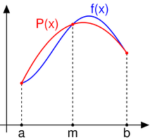
In the figure, f(x) implies the actual existing curve and P(x) is parabolic approximation of between two intervals.
Assume, Initial value of abscissa, x0 = a and Final value of abscissa, xn = b
Let m be a value of abscissa such that, m = ( a + b ) / 2
By using Lagrange Polynomial Interpolation, the expression for P(x) can be given as:
P(x) = f(a) [ (x-m) ( x-b ) ]/ [ (a-m) ( a-b)] + f(m) [(x-a) (x-b) ]/ [ (m – a) ( m – b) ]
+ f(b) [ (x – a) ( x – m ) ] / [ ( b – a ) ( b – m )]
Substitution of value of ‘m’ and integrating in the interval [a, b],
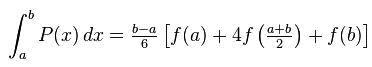
which is the required expression. The code of Simpson Rule in Matlab is based on this formula.
Simpson 1/3 Rule in MATLAB Code:
function I = simpson3_f ( f )
f = @(x) 2 + cos (2*sqrt(2))
% for calculating integrals using Simpson's 1/3 rule when function is known

%asking for the range and desired accuracy

 R= input( 'Enter the limits of integrations [ x_min, x_max]   :\n');
 tol = input('Error allowed in the final answer: \n');
 a= R(1,1); b = R(1,2);
 %intial h and n
 n = 100;
 h = (b -a )/100;
%for calculating maximum of f''''(x) in the given region

 for k = 0:100
        x( 1, k+1 ) = a +  k*h ;
        y4( 1, k+1) =    feval ( f, x(1,k+1) + 4*h ) - 4*feval( f, x(1,k+1) + 3*h )...
                                + 6*feval( f, x(k+1) + 2*h ) - 4* feval ( f, x(1,k+1) + h ) ...
                                + feval( f, x(k+1) );% fourth order difference
 end
 [ y i ] =  max( y4);
 x_opt = x(1,i);

 % for calculating the desired value of h
 m=0;
 ddf = feval ( f, x_opt + 4*h ) - 4*feval( f, x_opt + 3*h )...
        + 6*feval( f, x_opt + 2*h ) - 4* feval ( f, x_opt + h ) ...
        + feval( f, x_opt );% fourth order difference
    % dff defined outside bracket just for convinence
 while ddf * ( b -a )/180 > tol % error for Simpson's 1by3  rule
                m = m +1;
                h = h*10^-m;
                 ddf = feval ( f, x_opt + 4*h ) - 4*feval( f, x_opt + 3*h )...
                           + 6*feval( f, x_opt + 2*h ) - 4* feval ( f, x_opt + h ) ...
                           + feval( f, x_opt );% defined here for looping
 end

 %calculating  n
 n = ceil(  (b-a)/h );
 if rem( n,2) == 0
     n = n+1;
 end
 h = ( b-a )/n;
% calculating matrix X

 for k = 1:(n+1)
    X(k,1) = a + (k-1)*h;
    X(k,2) =feval ( f, X(k,1));
 end
%calculating integration

i= 1; I1 = 0;
while ( 2*i ) < (n+1)
    I1 =  I1 + X ( ( 2*i) , 2 );
    i = i +1;
end
j=1; I2 =0;
while (2*j + 1) < (n+1)
    I2 = I2 + X ( ( 2*j + 1)  , 2);
    j = j + 1;
end
I = h/3 * (  X( 1,2) +  4*I1  +  2*I2 +  X(n,2)  );% Simpson's 1/3 rule
% Display final result

h
n
disp(sprintf(' Using this integration for the given function in the range ( %10f , %10f )  is %10.6f .',a,b,I))
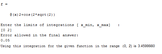
The above Matlab code is for Simpson’s 1/3 rule to evaluate the function f(x) = 2 + cos(2 ). If the code is to be used to evaluate the numerical integration of other integrands, the value of ‘f’ in the program can be modified as per requirement.
In this MATLAB program, the interval in which the numerical integration is to be carried out and the allowed error or tolerance are the input. After giving these inputs to the program, the value of numerical integration of the function is displayed on the screen.
A sample input/output screenshot of the program is given below:
Numerical Example of Simpson 1/3 Rule:
Now, let’s analyze mathematically the above program of Simpson rule in Matlab using the same function and limits of integration. The question here is:
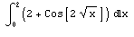
Evaluate the following integral by using Simpson 1/3 rule with m = 1 and 2.
Solution:
The given integrand is : f(x) = 2 + cos(2 )
The graph of f(x) can be shown as:
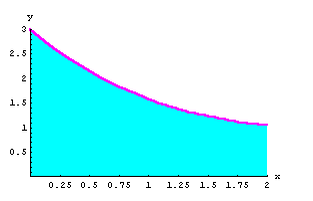
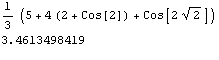
When m =1, using the expression for Simpson’s 1/3 rule:
I =
When m =2
I =
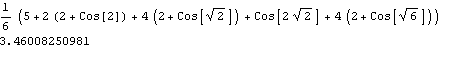
which is nearly the same as the value obtained from Simpson’s Matlab program.
If you have any questions regarding Simpson’s rule/method, its Matlab code, or mathematical derivation, bring them up from the comments. You can find more Numerical Methods tutorial using Matlab here.