Bisection Method

C Program

Bisection method is an iterative implementation of the ‘Intermediate Value Theorem‘ to find the real roots of a nonlinear function. According to the theorem “If a function f(x)=0 is continuous in an interval (a,b), such that f(a) and f(b) are of opposite nature or opposite signs, then there exists at least one or an odd number of roots between a and b.”
Using C program for bisection method is one of the simplest computer programming approach to find the solution of nonlinear equations. It requires two initial guesses and is a closed bracket method. Bisection method never fails!
The programming effort for Bisection Method in C language is simple and easy. The convergence is linear, slow but steady. The overall accuracy obtained is very good, so bisection method is more reliable in comparison to the Newton Raphson method or the Regula-Falsi method.

Features of Bisection Method:

• Type – closed bracket
• No. of initial guesses – 2
• Convergence – linear
• Rate of convergence – slow but steady
• Accuracy – good
• Programming effort – easy
• Approach – middle point

Below is a source code in C program for bisection method to find a root of the nonlinear function x^3 – 4*x – 9. The initial guesses taken are a and b. The calculation is done until the following condition is satisfied:
|a-b| < 0.0005 OR If (a+b)/2 < 0.0005 (or both equal to zero) where, (a+b)/2 is the middle point value.

Variables:

• itr – a counter variable which keeps track of the no. of iterations performed
• maxmitr – maximum number of iterations to be performed
• x – the value of root at the nth iteration
• a, b – the limits within which the root lies
• allerr – allowed error
• x1 – the value of root at (n+1)th iteration

#include< stdio.h>
#include< math.h>
float fun (float x)
{
    return (x*x*x - 4*x - 9);
}
void bisection (float *x, float a, float b, int *itr)
/* this function performs and prints the result of one iteration */
{
    *x=(a+b)/2;
    ++(*itr);
    printf("Iteration no. %3d X = %7.5f\n", *itr, *x);
}
void main ()
{
    int itr = 0, maxmitr;
    float x, a, b, allerr, x1;
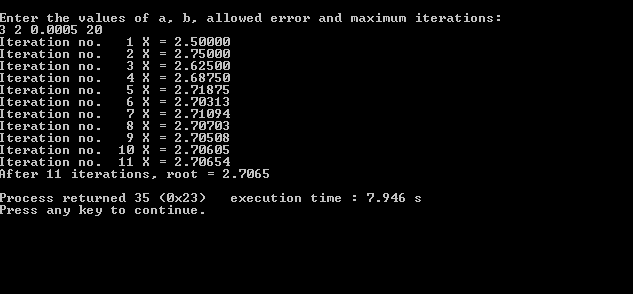
    printf("\nEnter the values of a, b, allowed error and maximum iterations:\n");
    scanf("%f %f %f %d", &a, &b, &allerr, &maxmitr);
    bisection (&x, a, b, &itr);
    do
    {
        if (fun(a)*fun(x) < 0)
            b=x;
        else
            a=x;
        bisection (&x1, a, b, &itr);
        if (fabs(x1-x) < allerr)
        {
            printf("After %d iterations, root = %6.4f\n", itr, x1);
            return 0;
        }
        x=x1;
    }
    while (itr < maxmitr);
    printf("The solution does not converge or iterations are not sufficient");
    return 1;
}

Input/Output:

MATLAB Program

Bisection method is a popular root finding method of mathematics and numerical methods. This method is applicable to find the root of any polynomial equation f(x) = 0, provided that the roots lie within the interval [a, b] and f(x) is continuous in the interval.
This method is closed bracket type, requiring two initial guesses. The convergence is linear and it gives good accuracy overall. Compared to other rooting finding methods, bisection method is considered to be relatively slow because of its slow and steady rate of convergence.
Earlier we discussed a C program and algorithm/flowchart of bisection method. Here, we’re going to write a source code for Bisection method in MATLAB, with program output and a numerical example.

Bisection Method Theory:

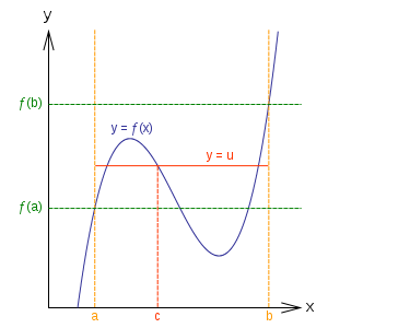
Bisection method is based on Intermediate Value Theorem. According to the theorem: “If there exists a continuous function f(x) in the interval [a, b] and c is any number between f(a) and f(b), then there exists at least one number x in that interval such that f(x) = c.”
The intermediate value theorem can be presented graphically as follows:

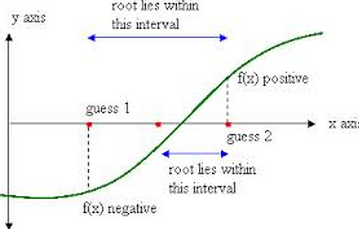
Here’s how the iteration procedure is carried out in bisection method (and the MATLAB program):

The first step in iteration is to calculate the mid-point of the interval [ a, b ]. If c be the mid-point of the interval, it can be defined as:

c = ( a+b)/2

The function is evaluated at ‘c’, which means f(c) is calculated. Now, three cases may arise:

• f(c) = 0 : c is the required root of the equation.
• f(b) * f(c) > 0 : if the product of f(b) and f(c) is positive, the root lies in the interval [a, c].
• f(b) * f(c) < 0 : if the product of f(b) and f(c) is negative, the root lies in the interval [ b, c].

In the second iteration, the intermediate value theorem is applied either in [a, c] or [ b, c], depending on the location of roots. And then, the iteration process is repeated by updating new values of a and b. The program for bisection method in MATLAB works in similar manner.

Bisection Method in MATLAB Code:

% Bisection Method in MATLAB
 
a=input('Enter function with right hand side zero:','s');
f=inline(a);
 
xl=input('Enter the first value of guess interval:') ;
xu=input('Enter the end value of guess interval:');
tol=input('Enter the allowed error:');
 
if f(xu)*f(xl)< 0
else
    fprintf('The guess is incorrect! Enter new guesses\n');
    xl=input('Enter the first value of guess interval:\n') ;
    xu=input('Enter the end value of guess interval:\n');
end
 
for i=2:1000
xr=(xu+xl)/2;
if f(xu)*f(xr)< 0
    xl=xr;
else
    xu=xr;
end
 
if f(xl)*f(xr)< 0
    xu=xr;
else
    xl=xr;
end
 
xnew(1)=0;
xnew(i)=xr;
if abs((xnew(i)-xnew(i-1))/xnew(i))< tol,break,end
end
str = ['The required root of the equation is: ', num2str(xr), '']

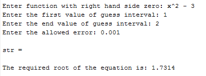
In this code for bisection method in Matlab, first the equation to be solved is defined, and it is then assigned with a variable f using inline() command. The program then asks for the values of guess intervals and allowable error.
The iteration process is similar to that described in the theory above. Or, you can go through this algorithm to see how the iteration is done in bisection method. Iteration continues till the desired root is allocated within the allowable error.
Here’s a sample output of this MATLAB program:

Bisection Method Example:

Now, lets analyze the above program of bisection method in Matlab mathematically. We have to find the root of x2 -3 = 0, starting with the interval [1, 2] and tolerable error 0.01.
Given that, f(x) = x2 -3 and a =1 & b =2
Mid-value of the interval, c = (a+b)/2 = (a+2)/2 = 1.5
f(c) = 1.52 -3 = -0.75
Check for the following cases:

• f(c) ≠ 0 : c is not the root of given equation.
• f(c ) * f(a) = -0.75 * -2 = 1.5 > 0 : root doesn’t lie in [1, 1.5]
• f(c ) * f( b) = -0.75 * 1= -0.75 < 0 : root lies in [1.5, 2]

The process is then repeated for the new interval [1.5, 2]. The table shows the entire iteration procedure of bisection method and its MATLAB program:

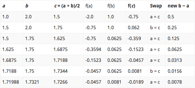
Thus, the root of x2 -3 = 0 is 1.7321. It is slightly different from the one obtained using MATLAB program. But, this root can be further refined by changing the tolerable error and hence the number of iteration.
If you have any questions regarding bisection method or its MATLAB code, bring them up from the comments. You can find more Numerical methods tutorial using MATLAB here.

Algorithm and Flowchart

Bisection method is used to find the real roots of a nonlinear equation. The process is based on the ‘Intermediate Value Theorem‘. According to the theorem “If a function f(x)=0 is continuous in an interval (a,b), such that f(a) and f(b) are of opposite nature or opposite signs, then there exists at least one or an odd number of roots between a and b.” In this post, the algorithm and flowchart for bisection method has been presented along with its salient features. Bisection method is a closed bracket method and requires two initial guesses. It is the simplest method with slow but steady rate of convergence. It never fails! The overall accuracy obtained is very good, so it is more reliable in comparison to the Regula-Falsi method or the Newton-Raphson method.

Features of Bisection Method:

• Type – closed bracket
• No. of initial guesses – 2
• Convergence – linear
• Rate of convergence – slow but steady
• Accuracy – good
• Programming effort – easy
• Approach – middle point

Bisection Method Algorithm:

• Start
• Read x1, x2, e
  *Here x1 and x2 are initial guesses
  e is the absolute error i.e. the desired degree of accuracy*
• Compute: f1 = f(x1) and f2 = f(x2)
• If (f1*f2) > 0, then display initial guesses are wrong and goto (11).
  Otherwise continue.
• x = (x1 + x2)/2
• If ( [ (x1 – x2)/x ] < e ), then display x and goto (11).
  * Here [ ] refers to the modulus sign. *
• Else, f = f(x)
• If ((f*f1) > 0), then x1 = x and f1 = f.
• Else, x2 = x and f2 = f.
• Goto (5).
  *Now the loop continues with new values.*
• Stop

Bisection Method Flowchart:

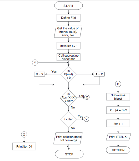
The algorithm and flowchart presented above can be used to understand how bisection method works and to write program for bisection method in any programming language.

Note: Bisection method guarantees the convergence of a function f(x) if it is continuous on the interval [a,b] (denoted by x1 and x2 in the above algorithm. For this, f(a) and f(b) should be of opposite nature i.e. opposite signs.
The slow convergence in bisection method is due to the fact that the absolute error is halved at each step. Due to this the method undergoes linear convergence, which is comparatively slower than the Newton-Raphson method, Secant method and False Position method.