Runge Kutta Method

C Program

A number of ordinary differential equations come in engineering and all of them may not be solved by analytical method. In order to solve or get numerical solution of such ordinary differential equations, Runge Kutta method is one of the widely used methods.
Unlike like Taylor’s series, in which much labor is involved in finding the higher order derivatives, in RK4 method, calculation of such higher order derivatives is not required. (Derivation)
This C program for Runge Kutta 4 method is designed to find out the numerical solution of a first order differential equation. It is a kind of initial value problem in which initial conditions are known, i.e the values of x0 and y0 are known, and the values of y at different values x is to be found out.
The source code below to solve ordinary differential equations of first order by RK4 method first asks for the values of initial condition i.e. user needs to input x0 and y0 . Then, the user has to define increment ‘h’ and the final value of x at which y is to be determined.
In this program for Runge Kutta method in C, a function f(x,y) is defined to calculate slope whenever it is called.

Source Code for Runge Kutta Method in C:

#include< stdio.h>
#include< math.h>
float f(float x,float y);
int main()
{
    float x0,y0,m1,m2,m3,m4,m,y,x,h,xn;
    printf("Enter x0,y0,xn,h:");
    scanf("%f %f %f %f",&x0,&y0,&xn,&h);
    x=x0;
    y=y0;
    printf("\n\nX\t\tY\n");
    while(x< xn)
    {
        m1=f(x0,y0);
        m2=f((x0+h/2.0),(y0+m1*h/2.0));
        m3=f((x0+h/2.0),(y0+m2*h/2.0));
        m4=f((x0+h),(y0+m3*h));
        m=((m1+2*m2+2*m3+m4)/6);
        y=y+m*h;
        x=x+h;
        printf("%f\t%f\n",x,y);
    }
}
float f(float x,float y)
{
    float m;
    m=(x-y)/(x+y);
    return m;
}

Input/Output:

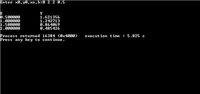
The above C program for Runge Kutta 4 method and the RK4 method itself gives higher accuracy than the inconvenient Taylor’s series; the accuracy obtained agrees up to the term h^r, where r varies for different methods, and is defined as the order of that method.
The RK formulas require the values of function at some selected points only. Further, Euler’s method is the Runge Kutta method of first order.

MATLAB Program

Runge-Kutta method is a popular iteration method of approximating solution of ordinary differential equations. Developed around 1900 by German mathematicians C.Runge and M. W. Kutta, this method is applicable to both families of explicit and implicit functions. Also known as RK method, the Runge-Kutta method is based on solution procedure of initial value problem in which the initial conditions are known. Based on the order of differential equation, there are different Runge-Kutta methods which are commonly referred to as: RK2, RK3, and RK4 methods. In earlier tutorial, we’ve already discussed a C program for RK4 method. This tutorial focuses on writing a general program code for Runge-Kutta method in MATLAB along with its mathematical derivation and a numerical example.

Derivation of Runge-Kutta Method:

Let’s consider an initial value problem given as:
y’ = f( t, y), y(t0) = y0
where,

• y is an unknown function of time t, which may be scalar or vector quantity
• y’ is the rate of change of y with respect to t
• t0 is the initial value of t
• y0 is the value of y at time t0

Let ‘h’ be the step size such that h > 0. Now, the generation term of the series can be defined as:
yn+1 = yn + h/6 * ( k1 + 2k2 + 2k3 + k4)
tn+1 = tn + h
for n = 1, 2 , 3, 4, …. such that:

• k1 = f( tn, yn)
• k2 = f( tn + h/2 , yn + h/2 k1 )
• k3 = f( tn + h/2, yn + h/2k2)
• k4 = f( tn + h, yn + hk3)
• yn+1 is the Runge-Kutta method approximation of y(tn+1)
• k1 is the increment which depends on the gradient of starting interval as in Euler’s method
• k2 is the increment which relies on the slope at the midpoint of the interval, k2 = y+ h/2 * k1
• k3 is also an increment based on the gradient at midpoint, k3=y+h/2*k2
• k4 is again an increment whose value depends on end of the end of interval k4 = y + hk3

Runge-Kutta Method in MATLAB:

function a = runge_kutta(df)
% asking initial conditions
 
x0 = input('Enter initial value of x : ');
y0 = input ('Enter initial value of y : ');
x1 = input( 'Enter value of x at which y is to be calculated : ');
tol = input( 'Enter desired level of accuracy in the final result : ');
 
%choose the order of Runge-Kutta method
 
r = menu ( ' Which order of Runge Kutta u want to use', ...
 ' 2nd order ' , ' 3rd order ' , ' 4th order ');
 
switch r
 case 1
 % calculating the value of h
 n =ceil( (x1-x0)/sqrt(tol));
 h = ( x1 - x0)/n;
 for i = 1 : n
 X(1,1) = x0; Y (1,1) = y0;
 k1 = h*feval( df , X(1,i), Y(1,i));
 k2 = h*feval( df , X(1,i) + h , Y(1,i) + k1);
 k = 1/2* ( k1+ k2);
 X( 1, i+1) = X(1,i) + h;
 Y( 1 ,i+1) = Y(1,i) + k;
 end
 
 case 2
 % calculating the value of h
 n =ceil( (x1-x0)/nthroot(tol,3));
 h = ( x1 - x0)/n;
 for i = 1 : n
 X(1,1) = x0; Y (1,1) = y0;
 k1 = h*feval( df , X(1,i), Y(1,i));
 k2 = h*feval( df , X(1,i) + h/2, Y(1,i) + k1);
 k3 = h*feval( df , X(1,i) + h, Y(1,i) + k2);
 k = 1/6* ( k1+ 4*k2 + k3);
 X( 1, i+1) = X(1,i) + h;
 Y( 1 ,i+1) = Y(1,i) + k;
 end
 
 case 3
 % calculating the value of h
 n =ceil( (x1-x0)/nthroot(tol,3));
 h = ( x1 - x0)/n;
 for i = 1 : n
 X(1,1) = x0; Y (1,1) = y0;
 k1 = h*feval( df , X(1,i), Y(1,i));
 k2 = h*feval( df , X(1,i) + h/2, Y(1,i) + k1);
 k3 = h*feval( df , X(1,i) + h/2, Y(1,i) + k2);
 k4 = h*feval( df , X(1,i) + h, Y(1,i) + k3);
 k = 1/6* ( k1+ 2*k2 + 2*k3 + k4);
 X( 1, i+1) = X(1,i) + h;
 Y( 1 ,i+1) = Y(1,i) + k;
 end
 
end
 
%displaying results
 
fprintf( 'for x = %g \n y = %g \n' , x1,Y(1,n+1))
 
%displaying graph
 
x = 1:n+1;
y = Y(1,n+1)*ones(1,n+1) - Y(1,:);
plot(x,y,'r')
xlabel = (' no of interval ');
ylabel = ( ' Error ');

The given code for Runge-Kutta method in Matlab is applicable to find out the approximate solution of ordinary differential equation of any order. In the source code, the argument ‘df’ is defined to represent equation, making right hand side zero.
The differential equation to be solved is given as input to the program through a MATLAB file. For example, if y ‘ = sin(x) + 2 is to be solved by using this MATLAB source code, following piece of codes should be saved as ex.m file and opened while executing the above program:

2
3
4
% y is the function of x alone 
 
function y=y(x)
y=sin (x) +2 ;

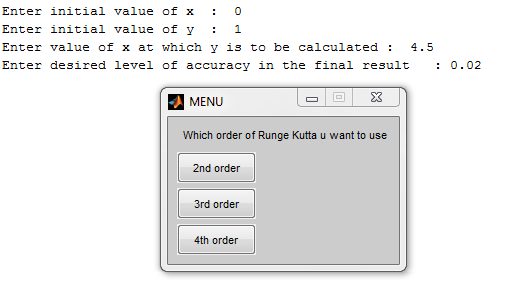
As the Runge-Kutta Methods are based on initial value problem, it is necessary to define the initial condition in any problem. When the program is executed, it asks for initial condition i.e. initial value of x, initial value of y, and the degree of accuracy or error tolerance.
After inputting all the values, the program asks to choose the order of Runge-Kutta method. Based on the order, the calculations are proceeded as explained above in the mathematical derivation. Here’s a sample output of the program:

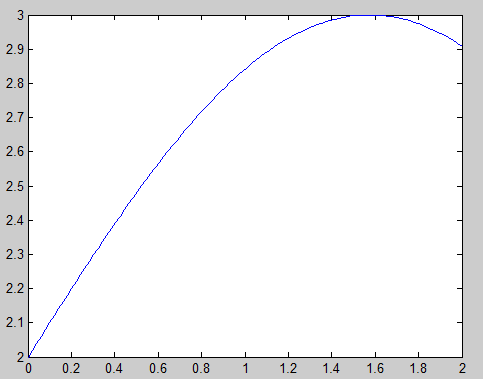
The last part of the code is for displaying graph as shown below:

Runge-Kutta Numerical Example:

Let’s analyze and solve an initial value problem using Runge-Kutta method. We have to approximate y(1.5) and y(1.0) using RK4 method in this problem:
y'(t) = 1 – t*y(t) ; y(0.5) = 2.5
Here, given initial condition: t0 = 0.5, y0 = 2.5
For y’ = 1 – ty, adopt a step size, h = 1. Then, finding the value of k1, k2, k3 and k4 using the formulas discussed in the derivation.

K1 = f(0.5, 2.5) = -0.25
K2 = f(1, 2.375) = -1.375
K3 = f(1, 1.8125) = -0.8125
K4 = f(0.5, 1.6875) = -0.153125
(K1 + 2K2 + 2K3 + K4)/6 = -1.026041667

The first approximation of y, y1 = y0 + h(-1.026041667) = 1.473958333

Next, to approximate y2, we have: t0 = 0.5, y0 = 2.5, and h = 0.5
K1 = f(0.5, 2.5) = -0.25
K2 = f(1, 2.4375) = -0.828125
K3 = f(1, 2.29296875) = -0.719726562
K4 = f(0.5, 2.140136719) = -1.140136719
(K1 + 2K2 + 2K3 + K4)/6 = -0.7476399739
The second approximation of y, y2 = y0 + h(-0.7476399739) = 2.126180013 …. and so on for others.
The whole calculation procedure of this numerical example (and of any program code of Runge-Kutta method in MATLAB) is shown in the table below:

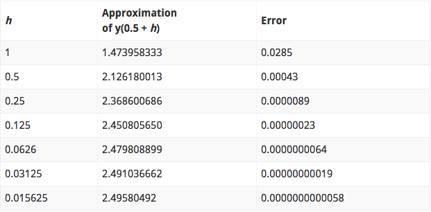
In Runge-Kutta method, the accuracy of the result depends on the value of step size, h. Smaller the value of h, higher will be the accuracy of the result obtained. The aforementioned table shows the various value of h in descending order and respective result of the function.
So, whether you’re solving a program manually or by programming (using MATLAB, C, or any other language syntax), the smaller the value of h, smaller will be the error in calculation of result. You can find more Numerical methods tutorial using MATLAB here.