Gauss Seidal/Jacobi Method

C Program

The direct methods such as Cramer’s rule, matrix inversion method, Gauss Elimination method, etc. for the solution of simultaneous algebraic equations yield the solution after a certain amount of fixed computation. So, direct method of solution takes longer time to get the solution.
On the other hand, in case of iterative methods such as Gauss Jacobi and Gauss-Seidel iteration method, we start with an approximate solution of equation and iterate it till we don’t get the result of desired accuracy. Here is source code for Gauss-Seidel in C with working procedure and sample output.
The manual computation iterative method is quite lengthy. But, the program in high level languages run fast and effectively. This C program for Gauss-Seidel method has been designed for the solution of linear simultaneous algebraic equations based on the principle of iteration.
In this program, a certain approximate value of solution is assumed and further calculations are done based on the result of assumed approximate solution.
The program for Gauss-Seidel method in C works by following the steps listed below:

• When the program is executed, first of all it asks for the value of elements of the augmented matrix row wise.
• Then, the program asks for allowed error and maximum number of iteration to which the calculations are to be done. The number of iterations required depends upon the degree of accuracy.
• The program assumes initial or approximate solution as y=0 and z=0 and new value of x which is used to calculate new values of y and z using the following expressions:

• The iteration process is continued until a desired degree of accuracy is not met.

Source Code for Gauss-Seidel Method in C:

#include
#include
#define X 2
main()
{
    float x[X][X+1],a[X], ae, max,t,s,e;
    int i,j,r,mxit;
    for(i=0;i< X;i++) a[i]=0;
    puts(" Eneter the elemrnts of augmented matrix rowwise\n");
    for(i=0;i< X;i++)
    {
    for(j=0;j< X+1;j++)
    {
    scanf("%f",&x[i][j]);
    }
    }
    printf(" Eneter the allowed error and maximum number of iteration: ");
    scanf("%f%d",&ae,&mxit);
    printf("Iteration\tx[1]\tx[2]\n");
    for(r=1;r<=mxit;r++)
    {
        max=0;
        for(i=0;i< X;i++)
        {
            s=0;
            for(j=0;j< X;j++)
            if(j!=i) s+=x[i][j]*a[j];
            t=(x[i][X]-s)/x[i][i];
            e=fabs(a[i]-t);
            a[i]=t;
        }
        printf(" %5d\t",r);
        for(i=0;i< X;i++)
        printf(" %9.4f\t",a[i]);
        printf("\n");
        if(max< ae)
        {
            printf(" Converses in %3d iteration\n", r);
            for(i=0;i< X;i++)
            printf("a[%3d]=%7.4f\n", i+1,a[i]);
            return 0;
        }
 
        }
    }

Input/Output:

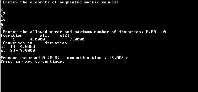
In this C language code for Gauss-Seidel method, the value of order of square matrix has been defined as a macro of value 2 which can be changed to any order in the source code.
Also, the elements of augmented matrix have been defined as array so that a number of values can be stored under a single variable name. The program can be used effectively to solve linear simultaneous algebraic equation though easy, accurate and convenient way.

MATLAB Program

Gauss-Seidel method is a popular iterative method of solving linear system of algebraic equations. It is applicable to any converging matrix with non-zero elements on diagonal. The method is named after two German mathematicians: Carl Friedrich Gauss and Philipp Ludwig von Seidel.
Gauss-Seidel is considered an improvement over Gauss Jacobi Method. In this method, just like any other iterative method, an approximate solution of the given equations is assumed, and iteration is done until the desired degree of accuracy is obtained.
In earlier tutorials, we’ve already gone through the C program and algorithm/flowchart for Gauss-Seidel method. Here, we’re going to write a program code for Gauss-Seidel method in MATLAB, discuss its theoretical background, and analyze the MATLAB program’s result with a numerical example.

Gauss-Seidel Method Theory:

Let’s go through a brief theoretical/mathematical background of Gauss-Seidel method. The matrices, iterations, and the procedure explained below cover the basic guidelines to write the program code for Gauss-Seidel method in MATLAB.

Consider the following system of linear equations:

a11x1 + a12x2 + a13x3 + a14x4 + a15x5 + a16x6 ……. + a1nxn = b1
a21x1 + a22x2 + a23x3 + a24x4 + a25x5 + a26x6 ……. + a2nxn = b2
a31x1 + a32x2 + a33x3 + a34x4 + a35x5 + a36x6 ……. + a3nxn = b3
. . . . . . . . . . . . . . . . . . . . . . . . . . . . . . . ….. . . . . . . . .. . . . . . . . . . . . . .. . . .. . . .
. . . . . . . . . . . . . . . . . . . . . . . . . . . . . . . ….. . . . . . . . .. . . . . . . . . . . . . .. . . .. . . .
an1x1 + an2x2 + an3x3 + an4x4 + an5x5 + an6x6 ……. + annxn = bn

where, aij represents the coefficient of unknown terms xi.

The above equations can be presented in matrix form as follows:

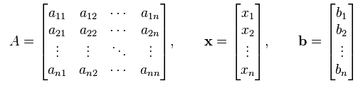
Or simply, it can be written as: [A][X] = [B]

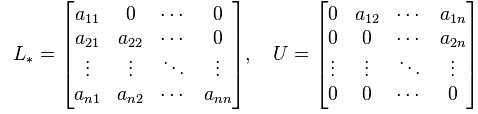
Now, decomposing the matrix A into its lower triangular component and upper triangular component, we get:

A = L x U

where,

Further, the system of linear equations can be expressed as:

L x X = B – UX —–(a)

In Gauss-Seidel method, the equation (a) is solved iteratively by solving the left hand value of x and then using previously found x on right hand side. Mathematically, the iteration process in Gauss-Seidel method can be expressed as:

X(k+1) = L -1( B –UX(k) )

Applying forward substitution, the elements of X(k+1) can be computed as follows:

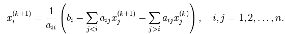
The same procedure aforementioned is followed in the MATLAB program for this method. The process of iteration is continued till the values of unknowns are under the limit of desired tolerance.

Gauss-Seidel Method in MATLAB:

% Gauss-Seidel Method in MATLAB
 
function x = gauss_siedel( A ,B )
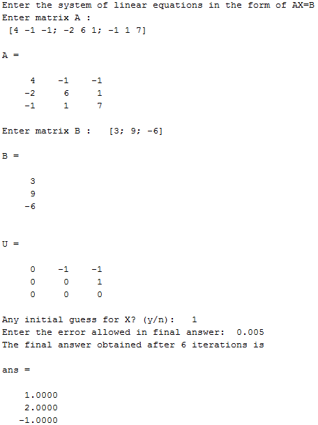
disp ( 'Enter the system of linear equations in the form of AX=B')
 
%Inputting matrix A
 
A = input ( 'Enter matrix A :   \n')
% check if the entered matrix is a square matrix
 
[na , ma ] = size (A);
if na ~= ma
    disp('ERROR: Matrix A must be a square matrix')
    return
end
 
% Inputting matrix B
 
B = input ( 'Enter matrix B :   ')
% check if B is a column matrix
 
[nb , mb ] = size (B);
if nb ~= na || mb~=1
   disp( 'ERROR: Matrix B must be a column matrix')
   return
end
 
% Separation of matrix A into lower triangular and upper triangular matrices
 
% A = D + L + U
 
D = diag(diag(A));
L = tril(A)- D;
U = triu(A)- D
 
% check for convergence condition for Gauss-Seidel method
 
e= max(eig(-inv(D+L)*(U)));
if abs(e) >= 1
    disp ('Since the modulus of the largest Eigen value of iterative matrix is not less than 1') 
    disp ('this process is not convergent.')
    return
end
 
% initial guess for X..?
 
% default guess is [ 1 1 .... 1]
 
r = input ( 'Any initial guess for X? (y/n):   ','s');
switch r 
    case 'y'
        % asking for initial guess
    X0 = input('Enter initial guess for X :\n')
        % check for initial guess
    [nx, mx] = size(X0);
        if nx ~= na || mx ~= 1
        disp( 'ERROR: Check input')
        return
    end
    otherwise
    X0 = ones(na,1);
end
 
% allowable error in final answer
 
t = input ( 'Enter the error allowed in final answer:  ');
tol = t*ones(na,1);
k= 1;
 
X( : , 1 ) = X0;
err= 1000000000*rand(na,1);% initial error assumption for looping
while sum(abs(err) >= tol) ~= zeros(na,1)
    X ( : ,k+ 1 ) = -inv(D+L)*(U)*X( : ,k) + inv(D+L)*B;% Gauss-Seidel formula
    err = X( :,k+1) - X( :, k);% finding error
    k = k + 1;
    
end
 
fprintf ('The final answer obtained after %g iterations is  \n', k)
X( : ,k)

In the above MATLAB program, a function, x = gauss_siedel( A ,B ), is initially defined. Here, A and B are the matrices generated with the coefficients used in the linear system of equations. The elements of A and B are input into the program following the basic syntax of MATLAB programming.

A and B are to be checked: A should be a square matrix and B must be a column matrix to satisfy the criteria of Gauss-Seidel method. Then, as explained in the theory, matrix A is split into its upper triangular and lower triangular parts to get the value of first iteration.
The value of variables obtained from the first iteration are used to start the second iteration, and the program keeps on iterating till the solution are in the desired limit of tolerance as provided by the user.
Here’s a sample output screen of the MATLAB program:

Gauss-Seidel Method Example:

The above MATLAB program of Gauss-Seidel method in MATLAB is now solved here mathematically. The equations given are:

4x1 – x2 –x3 = 3
-2x1 + 6x2 + x3 = 9
-x1 + x2 – 7x3 = -6

In order to get the value of first iteration, express the given equations as follows:

4x1 – 0 –0 = 3
-2x1 + 6x2 + 0 = 9
-x1 + x2 – 7x3 = -6

From the first equation: x1 = 3/4 = 0.750
Substitute the value of x1 in the second equation : x2 = [9 + 2(0.750)] / 6 = 1.750
Substitute the values of x1 and x2 in the third equation: x3 = [-6 + 0.750 − 1.750] / 7 = − 1.000
Thus, the result of first iteration is: ( 0.750, 1.750, -1.000 )

The whole iteration procedure that goes on in Gauss-Seidel method (and the above MATLAB program) is presented below:

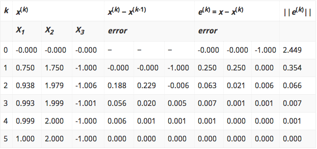
where, k is the number of iteration.

The final solution obtained is (1.000, 2.000, -1.000).

If you have any questions regarding Gauss-Seidel method, its theory, or MATLAB program, drop them in the comments. You can find more Numerical methods tutorial using MATLAB here.

Algorithm and Flowchart

Gauss-Seidel and Gauss Jacobi method are iterative methods used to find the solution of a system of linear simultaneous equations. Both are based on fixed point iteration method. Whether it’s a program, algorithm, or flowchart, we start with a guess solution of the given system of linear simultaneous equations, and iterate the equations till the desired degree of accuracy is reached.
In Gauss Jacobi method, we assume x1, x2 and x3 as the three initial guesses. To get better values, the approximations in previous iterations are used. In this method, we should see that the variable absolute value coefficient is greater than or equal to sum of the absolute values of the coefficient of the remaining variables.
Guass-Seidel method is very similar to Gauss Jacobi method, and here are simple algorithm and flowchart for Gauss-Seidel and Gauss Jacobi method. In Gauss Seidel method, the most recent values or fresher values are used in successive iterations.

Gauss-Seidel Method Algorithm:

• Start
• Declare the variables and read the order of the matrix n
• Read the stopping criteria er
• Read the coefficients aim as
  Do for i=1 to n
  Do for j=1 to n
  Read a[i][j]
  Repeat for j
  Repeat for i
• Read the coefficients b[i] for i=1 to n
• Initialize x0[i] = 0 for i=1 to n
• Set key=0
• For i=1 to n
  Set sum = b[i]
  For j=1 to n
  If (j not equal to i)
  Set sum = sum – a[i][j] * x0[j]
  Repeat j
  x[i] = sum/a[i][i]
  If absolute value of ((x[i] – x0[i]) / x[i]) > er, then
  Set key = 1
  Set x0[i] = x[i]
  Repeat i
• If key = 1, then
  Goto step 6
  Otherwise print results

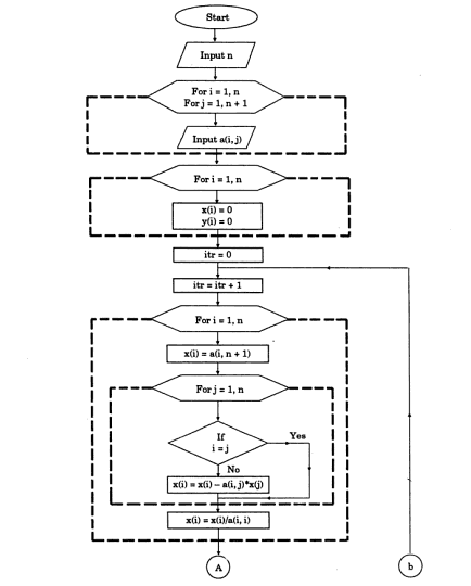
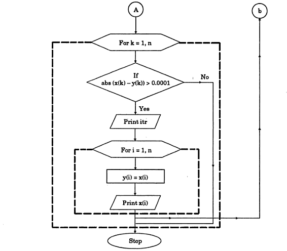
Gauss-Seidel Method Flowchart:

Gauss Jacobi Method Flowchart:

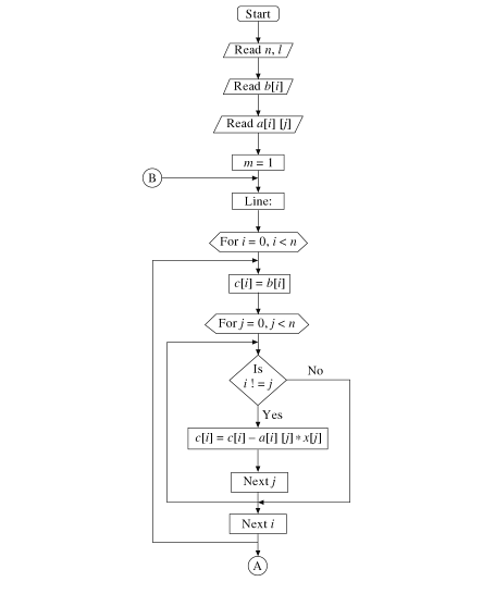
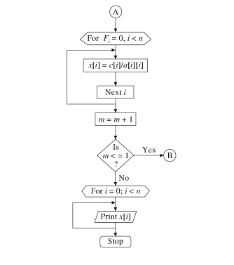
Programs in any high level programming language can be written with the help of these Gauss-Seidel and Gauss Jacobi method algorithm and flowchart to solve linear simultaneous equations.
This method is fast and easy compared to the direct methods such as Gauss Jordan method, Gauss Elimination method , Cramer’s rule, etc. However, the manual computation of Gauss Seidel/Jacobi method can also be lengthy.