Modified Euler’s Method

C Program

The analytical method of solution of differential equation is time consuming and tedious. Sometimes it fails to give accurate solution to complicated problems. In order to save time and labor, methods of numerical solution of differential equations such as Euler’s method, Modified Euler’s Method, Runge Kutta Method etc. have been developed.
Here, we are going to discuss a C program for Modified Euler’s method with its source code and sample output. The program is designed for numerical solution of ordinary differential equations or initial value problems in which all the initial conditions are specified.
The input data for Modified Euler’s Method in C given below are initial and final values of x i.e. x0 and xn, initial value of y i.e y0 and the value of increment i.e h.
Here’s how the C source code for Modified Euler’s method works:

• When the program is executed, it checks the error and if the program is found to be error free, the program runs. Firstly, it asks the value of initial condition i.e. initial value of x and y, value of increment h, and final value of x.
• After getting the initial condition, this C program calls the defined function float fun(float,float) for the calculation of slope. The function for calculation of slope is:-
  y’ = x2 + y
• Then, value of x is increased by h i.e. x1 = x0 + h and so on. Using the new value of x and y, new slope is calculated. Mean slope of this newly calculated and initial slope is calculated.
• The new value of y is : y= y0 + h * slope. The value of x is not increased till the any two consecutive value of y are found to be same or with the given limit of tolerance.
• The process is repeated till the initial value of x is not equal to the final value of x.
• Finally, the program prints the intermediate as well as final values of x and corresponding y. These values can be transferred to Curve Software to obtain curve and its equations.

Source Code for Modified Euler’s Method in C:

#include< stdio.h>
#include< math.h>
#include< string.h>
float fun(float,float);
main()
    {
        int i,j,c;
        float x[100],y[100],h,m[100],m1,m2,a,s[100],w;
        printf("\n     C program for Modified Euler Method \n\n");
        printf("  Enter the initial value of x:");
        scanf("%f",&x[0]);
        printf("\n  Enter the value of increment h:");
        scanf("%f",&h);
        printf("\n  Enter the final value of x:");
        scanf("%f",&a);
        printf("\n  Enter the initial value of the variable y :");
        scanf("%f",&y[0]);
        s[0]=y[0];
        for(i=1;x[i-1]< a;i++)
            {
                w=100.0;
               x[i]= x[i-1]+h;
               m[i]=fun(x[i-1],y[i-1]);
               c=0;
               while(w>0.0001)
                {
                    m1=fun(x[i],s[c]);
                    m2=(m[i]+m1)/2;
                    s[c+1]=y[i-1]+m2*h;
                    w=s[c]-s[c+1];
                    w=fabs(w);
                    c=c+1;
                }
              y[i]=s[c];
            }
        printf("\n\n The respective values of x and y are\n     x  \t     y\n\n");
        for(j=0;j< i;j++)
            {
                printf("  %f\t%f",x[j],y[j]);
                printf("\n");
            }
    }
float fun(float a,float b)
    {
        float c;
        c=a*a+b;
        return(c);
    }

Input/Output:

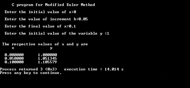
Smaller the value of h, higher will be the accuracy of the result obtained from this program for modified Euler’s method in C. This method was developed by Leonhard Euler during the 1770s. Modified Euler’s method gives greater improvement in accuracy over the Euler’s method; but it is a bit long and tedious to some extent.

MATLAB Program

Modified Euler’s Method is a popular method of numerical analysis for integration of initial value problem with the best accuracy and reliability. It solves ordinary differential equations (ODE) by approximating in an interval with slope as an arithmetic average. This method is a simple improvement on Euler’s method in function evaluation per step but leads to yield a second order method.
In earlier tutorials, we’ve already gone through a C program and algorithm/flowchart for this method. Here, we’re going to write a program for Modified Euler’s method in Matlab, and discuss its mathematical derivation and a numerical example.

Derivation of Modified Euler’s Method:

Consider y which is the function of t and solution to an ordinary differential equation. y can be graphically represented as follows:

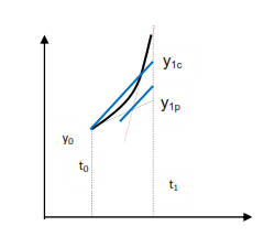
Let h be height of small intervals taken during the process of approximation.
h = (xn – x0)/n
We are provided y(t) as an initial value and we are to evaluate y(t+h)
By using Taylor’s Series:
y(t ) = y( t+ h ) – h [dy ( t + h )]/dt + h2/2 [d2y ( t + h )]/dt2 – O(h3)
Rearranging the terms:
y( t+ h ) = y (t ) + h [dy ( t + h )]/dt – h2/2 [d2y ( t + h )]/dt2 + O(h3)
Solving this equation:
y( t + h ) = y (t) + h/2 [ dy(t)/dt + dy (t +h ) / dt ] + O(h3)
The values of O(h3) and other higher terms are very small and generally neglected. Based on this derivation, we’ll work out the code for Modified Euler’s method in Matlab.

Modified Euler’s Method in MATLAB:

function a= eular(  df )
%df = @(x, y) -2xy^2
 
% for calculating value of dy/dx at some particular pt using modified euler's method
 
% asking intial conditions
 
x0 = input('Enter initial value of x  :  ');
y0 = input ('Enter initial value of y  :  ');
x1 = input( 'Enter thevalue of x at which y is to be calculated :  ');
tol = input( 'Enter desired level of accuracy in the final result   : ');
% calaulating the value of h
 
n =ceil( (x1-x0)/sqrt(tol));
h = ( x1 - x0)/n
%loop for calculating values
 
for k = 1 : n
    X(1,1) = x0; Y (1,1) = y0;
    X( 1, k+1) = X(1,k) + h;
    y_t = Y(1,k) + h* feval( df , X(1,k) , Y(1,k));% Eular's formula
    Y(1 ,k+1) = Y(1,k) + h/2* (feval( df , X(1,k) , Y(1,k)) + feval( df , X(1,k) + h , y_t ) ) ;
    %improving results obtained by modified Eular's formula
    while abs( Y(1,k+1) - y_t ) > h
        y_t = Y(1,k) + h*feval( df , X(1,k) , Y(1,k+1));
        Y( 1 ,k+1) = Y(1,k) + h/2* (feval( df , X(1,k) , Y(1,k)) + feval( df , X(1,k) + h , y_t ) );
    end
end
%displaying results
 
fprintf( 'for \t x = %g \n \ty = %g \n' , x1,Y(1,n+1))
%displaying graph
 
x = 1:n+1;
y = Y(1,n+1)*ones(1,n+1) - Y(1,:);
plot(x,y,'b')
xlabel = (' no of intarval ');
ylabel = ( ' Error ');

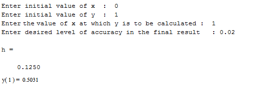
The above source code for Modified Euler’s Method in Matlab is written for solving ordinary differential equation: y’ = -2xy2 with the initial value condition that, x0 = 0 and y0 = 1. The program can be modified to solve any equation by changing the value of ‘df’ in the code. This code is a four-parameter input program: it needs initial value of x, initial value of y, the final value of x at which y is to be evaluated and allowed error as the inputs. When all the inputs are given to the program, it displays the value of step height, h and the final value of y at the desired x as output.

The sample output of the program for the function and initial value condition mentioned above is given below:

Numerical Example of Modified Euler’s Method:

Now, let’s analyze mathematically the above program code of Modified Euler’s method in Matlab. The questions here is:

Given function is, f(x, y) = -2xy2
Initial value condition, x0 = 0 and y0 = 1
Step height, h = 0.2
1. Approximation for y(t +h) i.e. y( 0 + 0.2) = y ( 0.2 )
y(1) = y(0) + 0 .5*h*((-2*x*y*y)(0) + (-2*x*y*y) (1)
y[0.20] = 1.0 * y[0.20] = 0.9599999988079071 * y[0.20] = 0.9631359989929199

y[0.20] = 0.9628947607919341 * y[0.20] = 0.9629133460803093

2. Approximation for y(t +h) i.e. y( 0.2 + 0.2) = y ( 0.4 )
y(2) = y(1) + 0 .5 * h * ((-2*x*y*y) (1) + (-2*x*y*y) (2)
y[0.40] = 0.8887359638083165 y[0.40] = 0.8626358081578545
y[0.40] = 0.8662926943348495 y[0.40] = 0.8657868947404332
y[0.40] = 0.865856981554814
3. Approximation for y(t +h) i.e. y( 0.4 + 0.2) = y ( 0.6 )
y(3) = y(2) + 0.5 * h* ((-2*x*y*y)(2) + (-2*x*y*y) (3)
y[0.60] = 0.7458966289094106 y[0.60] = 0.7391085349039348
y[0.60] = 0.7403181774980547 y[0.60] = 0.7401034281837107
y[0.60] = 0.7401415785278189
4. Approximation for y(t +h) i.e. y( 0.6 + 0.2) = y ( 0.8 )
y(4) = y(3) + 0 .5* h * ((-2*x*y*y) (3) + (-2* x* y* y) (4)
y[0.80] = 0.6086629119889084 y[0.80] = 0.6151235687114084
y[0.80] = 0.6138585343771569 y[0.80] = 0.6141072871136244
y[0.80] = 0.6140584135348263
5. Approximation for y(t +h) i.e. y( 0.8 + 0.2) = y ( 1.0 )
y(5) = y(4) + 0.5 * h * ((-2*x*y*y)(4) + (-2*x*y*y)(5)
y[1.00] = 0.49340256427369866 y[1.00] = 0.5050460713552334
y[1.00] = 0.5027209825340415 y[1.00] = 0.5031896121302805
y[1.00] = 0.5030953322323046 y[1.00] = 0.503114306721248

which is the required answer. It is same as that obtained from the program of Modified Euler’s method in Matlab.
If you’ve any questions regarding Modified Euler’s method, its MATLAB program, or its mathematical derivation, bring them up from the comments section. You can find more Numerical Methods tutorials using Matlab here.

Algorithm and Flowchart

As the name implies, Modified Euler’s Method is a modification of the original Euler’s method. It was developed by Leonhard Euler during the 1770s. It is one of the best methods to find the numerical solution of ordinary differential equation.
Unlike the analytical method, the numerical solution of ordinary differential equation by Modified Euler’s method is easy and simple to understand from both numerical and programming point of view. The analytical method is outdated, consuming a lot of time and the procedure is tedious.
Here, algorithm and flowchart modified Euler’s method have been presented in such a way that with the help of these you can write source code in any high level programming language.
For both algorithm and flowchart, the initial or the boundary conditions must be specified. The information required as the input data are the initial and final values of x i.e. x0 and xn, initial value of y i.e y0 and the value of increment i.e h.

Modified Euler’s Method Algorithm:

• Start
• Define function to calculate slope f(x,y)
• Declare variables
• Input the value of variable
• Find slope ( say m0) using initial values of x & y i.e f( x0 ,yo )
• Find new y, y = y0 + m0 * h
• Increase value of x, i.e x1 = x0 + h
• Find new slope ( say m’) using x1 and y
• Take the mean of m0 and m
• Again find ynew , and assign ynew with y
• Repeat from step 6 till two consecutive y are equal
• New, increase x and repeat from step 5 till x = xn
• Print x and corresponding y
• Stop

Modified Euler’s Method Flowchart:

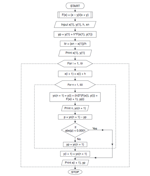
Analytical method often fails in case of complicated problems, but the modified Euler’s method does not fail, and gives higher degree of accuracy. It also gives improvement over the Euler’s method, though it may be somewhat long in coding. For higher degree of accuracy, you can choose the smaller values for h.
You can find complete source code, algorithm and flowchart for other methods to find solution of ordinary differential equation as well as the whole Numerical Methods course here. If you have any questions regarding Modified Euler’s method, its algorithm or flowchart, bring them up to me from the comments section.