Theoretical Paper
- Computer Organization
- Data Structure
- Digital Electronics
- Object Oriented Programming
- Discrete Mathematics
- Graph Theory
- Operating Systems
- Software Engineering
- Computer Graphics
- Database Management System
- Operation Research
- Computer Networking
- Image Processing
- Internet Technologies
- Micro Processor
- E-Commerce & ERP
Practical Paper
Industrial Training

SQL
Introduction
In this chapter, we shall learn more about the essentials of the relational model's standard language that will allow us to manipulate the data stored in the databases. This language is powerful yet flexible, thus making it popular. It is in fact one of the factors that has led to the dominance of the relational model in the database market today.
Following Codd's papers on the relational model and relational algebra and calculus languages, research communities were prompted to work on the realisation of these concepts. Several implemented versions of the relational languages were developed, amongst the most noted were SQL (Structured Query Language), QBE (Query-By- Example) and QUEL (Query Language). Here, we shall look into SQL with greater detail as it the most widely used relational language today. One often hears of remarks that say, "It's not relational if it doesn't use SQL". It is currently being standardised now as a standard language for the Relational Data Model.
SQL had its origins back in 1974 from IBM's System R research project as Structured English Query Language (or SEQueL) for use on the IBM VS/2 mainframes. It was developed by Chamberlain et al. The name was subsequently changed to Structured Query Language or SQL. It is pronounced "sequel" by some and S-Q-L by others. IBM's products such as SQL/DS and the popular DB2 emerged from this. SQL is based on the Relational Calculus with tuple variables. In 1986, the American National Standards Institute (ANSI) adopted SQL standards, contributing to its widespread adoption. Whilst many commercial SQL products exist with various "dialects", the basic command set and structure remain fairly standard.
The end user is given an interface, as we have seen in Chapter 3, to interact with the database via menus, query operations, report generators, etc. Behind this lies the SQL engine that performs the more difficult tasks of creating relation structures, maintaining the systems catalogues and data dictionary, etc.
SQL belongs to the category of the so-called Fourth-Generation Language (4GL) because of its power, conciseness and low-level of procedurality. As a non-procedural language it allows the user to specify what must be done without detailing how it must be done. The user's SQL request specification is then translated by the RDBMS into the technical details needed to get the required data. As a result, the relational database is said to require less programming than any other database or file system environment. This makes SQL relatively easy to learn.
Operations
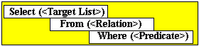
Mapping: The SQL Select Statement
The basic operation in SQL is called mapping, which transforms values from a database to user requirements. This operation is syntactically represented by the following block:
SQL Select
This uncomplicated structure can used to construct queries ranging from very simple inquiries to more complex ones by essentially defining the conditions of the predicate. It thus provides immense flexibility.
The SQL Select command combines the Relational Algebra operators Select, Project, Join and the Cartesian Product. Because a single declarative-style command can be used to retrieve virtually any stored data, it is also regarded by many to be an implementation of the Relational Calculus. If we need to extract information from only one relation of the database, we may encounter similarities and a few differences between the Relational Calculus-based DSL Alpha and SQL. In this case we may substitute key words of DSL Alpha for matching key words of SQL as follows:
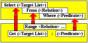
Similarities of DSL Alpha and SQL Select
Let us refer back to the earlier example with the Customer relation.
Suppose we wish to "Get the names and phone numbers of customers living in London". With DSL Alpha, we would specify this query as:
Range Customer X;
Get (X.Cname, X.Cphone): X.Ccity=London;
whereas in SQL its equivalent would be:
Select Cname, Phone
From Customer
Where Ccity = 'London
In either case, the result would be the retrieval of the following two tuples:
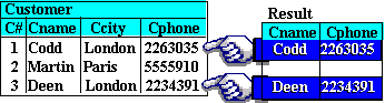
This simple query highlights the three most used SQL clauses:
1. The SELECT clause
This effectively gets the columns that we are interested in getting from the relation. We may be interested in a single column, thus we may for example write "Select Cphone" if we only wish to list just the telephone numbers. We may also however be interested in listing the customer's name, city and telephone number; in which case, we write "Select Cname, Ccity, Cphone".
2. The FROM clause
We need to identify the relations that our query refers to and this is done via the From clause. The columns that we have chosen from the Select clause must be found in the relation names of the From clause as in "From Customer".
3. The WHERE clause
This holds the conditions that allows us to restrict the tuples of the relation(s). In the example "Where Ccity=London" asserts that we wish to select only the tuples which contain the city name that is equal to the value 'London'.
The system first processes the From clause (and all tuples of the chosen relation(s) are placed in the processing work area), followed by the Where clause (which chooses, one by one, the tuples that satisfy the clause conditions and eliminating those which do not), and finally the Select clause (which takes the resultant tuples and displays only the values under the Select clause column names).
Output Restriction
Most queries do not need every tuple in the relation but rather only a subset of the tuples. As described previously in section 5.3, the following mathematical operators can be used in the predicate to restrict the output:
| Symbol | Meaning |
| = | Equal to |
| < | Less than |
| > | Greater than |
| <= | Less than or equal to |
| >= | Greater than or equal to |
< > |
Not equal to |
Additionally, the logical operators AND, OR and NOT may be used to place further restrictions. These logical operators, along with parentheses, may be combined to produce quite complex conditional expressions.
Suppose we need to retrieve the tuples from the Transaction relation such that the following conditions apply:
1. The transaction date is before 26 Jan and the quantity is at least 25
2. Or, the customer number is 2
The SQL statement that could get the desired result would be:
Select C#, Date, Qnt From Transaction
Where (Date < '26.01' And Qnt >= 25) Or C# = 2
9.2.3 Recursive Mapping: Sub-queries
The main idea of SQL is the recursive usage of the mapping operation instead of using the existential and universal quantifiers. So far in our examples, we always know the values that we want to put in our predicate. For example,
Where Ccity = 'London'
Where Date < '26.01' And Qnt > 25
Suppose we now wish to "Get the personal numbers of customers who bought the product CPU". We could start off by writing the SQL statement:
Select C#
From Transaction
Where P#= ?
We cannot of course write "Where P#=CPU" because CPU is a part name not its number. However as we may recall, part number P# is stored in the Transaction relation, but the part name is in fact in another relation, the Product relation.
Thus one needs to first of all get the part name from Product via another SQL statement:
Select P#
From Product
Where Pname = 'CPU'
Having obtained the equivalent P#, the value is then used to complete the earlier query. The way this is to be expressed is by writing the whole mapping operator in the right hand side of comparison expressions of another mapping operator. This effectively means the use of an inner block (sub-query) within the outer block (main query) as depicted in the figure below.
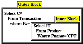
The query in the outer block thus executes by using the value set generated earlier by the sub-query of the inner block.
It is important to note that because the sub-query replaces the value in the predicate of the main query, the value retrieved from the sub-query must be of the same domain as the value in the main predicate.
Multiple Nesting
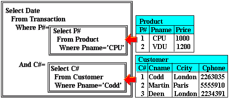
It is also possible that may be two or more inner blocks within an outer SQL block. For instance, we next wish to: `Get a date when customer Codd bought the product CPU.` The SQL statement we would start out with would probably look like this:
Select Date
From Transaction
Where P#=?
And C#=?
As in the earlier query , the part number P# can be obtained via the part name Pname in the relation Product. The customer name, Codd, however has to have its equivalent customer number which has to be obtained from C# of the relation Customer.
Thus to complete the above query, one would have to work two sub-queries first as follows:
 Interpretation of sub-queries
 Note that the original SQL notation utilises brackets or parentheses to determine inner SQL blocks as:
Select Date
From Transaction
Where P# =