File Management Systems Sequential Random Indexed Sequential Inverted

Relative data and information is stored collectively in file formats. A file is a sequence of records stored in binary format. A disk drive is formatted into several blocks that can store records. File records are mapped onto those disk blocks.

File Organization

File Organization defines how file records are mapped onto disk blocks. We have four types of File Organization to organize file records −

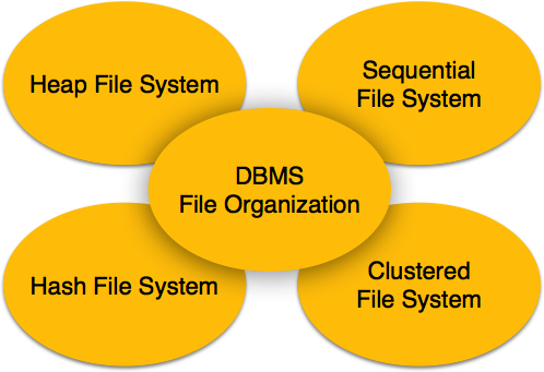
Heap File Organization

When a file is created using Heap File Organization, the Operating System allocates memory area to that file without any further accounting details. File records can be placed anywhere in that memory area. It is the responsibility of the software to manage the records. Heap File does not support any ordering, sequencing, or indexing on its own.

Sequential File Organization

Every file record contains a data field (attribute) to uniquely identify that record. In sequential file organization, records are placed in the file in some sequential order based on the unique key field or search key. Practically, it is not possible to store all the records sequentially in physical form.

Hash File Organization

Hash File Organization uses Hash function computation on some fields of the records. The output of the hash function determines the location of disk block where the records are to be placed.

Clustered File Organization

Clustered file organization is not considered good for large databases. In this mechanism, related records from one or more relations are kept in the same disk block, that is, the ordering of records is not based on primary key or search key.

File Operations

Operations on database files can be broadly classified into two categories −

• Update Operations

• Retrieval Operations

Update operations change the data values by insertion, deletion, or update. Retrieval operations, on the other hand, do not alter the data but retrieve them after optional conditional filtering. In both types of operations, selection plays a significant role. Other than creation and deletion of a file, there could be several operations, which can be done on files.

• Open − A file can be opened in one of the two modes, read mode or write mode. In read mode, the operating system does not allow anyone to alter data. In other words, data is read only. Files opened in read mode can be shared among several entities. Write mode allows data modification. Files opened in write mode can be read but cannot be shared.

• Locate − Every file has a file pointer, which tells the current position where the data is to be read or written. This pointer can be adjusted accordingly. Using find (seek) operation, it can be moved forward or backward.

• Read − By default, when files are opened in read mode, the file pointer points to the beginning of the file. There are options where the user can tell the operating system where to locate the file pointer at the time of opening a file. The very next data to the file pointer is read.

• Write − User can select to open a file in write mode, which enables them to edit its contents. It can be deletion, insertion, or modification. The file pointer can be located at the time of opening or can be dynamically changed if the operating system allows to do so.

• Close − This is the most important operation from the operating system’s point of view. When a request to close a file is generated, the operating system

  • removes all the locks (if in shared mode),
  • saves the data (if altered) to the secondary storage media, and
  • releases all the buffers and file handlers associated with the file.

The organization of data inside a file plays a major role here. The process to locate the file pointer to a desired record inside a file various based on whether the records are arranged sequentially or clustered.

We know that data is stored in the form of records. Every record has a key field, which helps it to be recognized uniquely.

Indexing is a data structure technique to efficiently retrieve records from the database files based on some attributes on which the indexing has been done. Indexing in database systems is similar to what we see in books.

Indexing is defined based on its indexing attributes. Indexing can be of the following types −

• Primary Index − Primary index is defined on an ordered data file. The data file is ordered on a key field. The key field is generally the primary key of the relation.

• Secondary Index − Secondary index may be generated from a field which is a candidate key and has a unique value in every record, or a non-key with duplicate values.

• Clustering Index − Clustering index is defined on an ordered data file. The data file is ordered on a non-key field.

Ordered Indexing is of two types −

• Dense Index
• Sparse Index

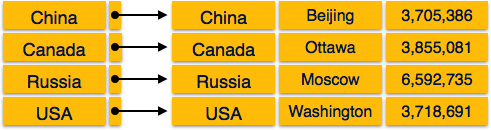
Dense Index

In dense index, there is an index record for every search key value in the database. This makes searching faster but requires more space to store index records itself. Index records contain search key value and a pointer to the actual record on the disk.

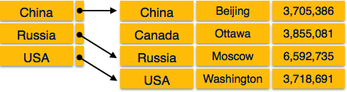
Sparse Index

In sparse index, index records are not created for every search key. An index record here contains a search key and an actual pointer to the data on the disk. To search a record, we first proceed by index record and reach at the actual location of the data. If the data we are looking for is not where we directly reach by following the index, then the system starts sequential search until the desired data is found.

Multilevel Index

Index records comprise search-key values and data pointers. Multilevel index is stored on the disk along with the actual database files. As the size of the database grows, so does the size of the indices. There is an immense need to keep the index records in the main memory so as to speed up the search operations. If single-level index is used, then a large size index cannot be kept in memory which leads to multiple disk accesses.

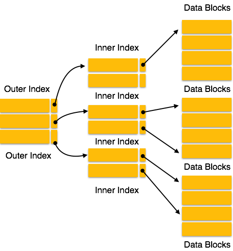
Multi-level Index helps in breaking down the index into several smaller indices in order to make the outermost level so small that it can be saved in a single disk block, which can easily be accommodated anywhere in the main memory.

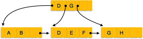
B⁺ Tree

A B⁺ tree is a balanced binary search tree that follows a multi-level index format. The leaf nodes of a B⁺ tree denote actual data pointers. B⁺ tree ensures that all leaf nodes remain at the same height, thus balanced. Additionally, the leaf nodes are linked using a link list; therefore, a B⁺ tree can support random access as well as sequential access.

Structure of B⁺ Tree

Every leaf node is at equal distance from the root node. A B⁺ tree is of the order n where n is fixed for every B⁺ tree.

Internal nodes −

• Internal (non-leaf) nodes contain at least ⌈n/2⌉ pointers, except the root node.
• At most, an internal node can contain n pointers.

Leaf nodes −

• Leaf nodes contain at least ⌈n/2⌉ record pointers and ⌈n/2⌉ key values.
• At most, a leaf node can contain n record pointers and n key values.
• Every leaf node contains one block pointer P to point to next leaf node and forms a linked list.

B⁺ Tree Insertion

• B⁺ trees are filled from bottom and each entry is done at the leaf node.

• If a leaf node overflows −

  • Split node into two parts.

  • Partition at i = ⌊(m+1)_/2⌋.

  • First i entries are stored in one node.

  • Rest of the entries (i+1 onwards) are moved to a new node.

  • i^th key is duplicated at the parent of the leaf.

• If a non-leaf node overflows −

  • Split node into two parts.

  • Partition the node at i = ⌈(m+1)_/2⌉.

  • Entries up to i are kept in one node.

  • Rest of the entries are moved to a new node.

B⁺ Tree Deletion

• B⁺ tree entries are deleted at the leaf nodes.

• The target entry is searched and deleted.

  • If it is an internal node, delete and replace with the entry from the left position.

• After deletion, underflow is tested,

  • If underflow occurs, distribute the entries from the nodes left to it.

• If distribution is not possible from left, then

  • Distribute from the nodes right to it.

• If distribution is not possible from left or from right, then

  • Merge the node with left and right to it.

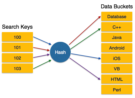
For a huge database structure, it can be almost next to impossible to search all the index values through all its level and then reach the destination data block to retrieve the desired data. Hashing is an effective technique to calculate the direct location of a data record on the disk without using index structure.

Hashing uses hash functions with search keys as parameters to generate the address of a data record.

Hash Organization

• Bucket − A hash file stores data in bucket format. Bucket is considered a unit of storage. A bucket typically stores one complete disk block, which in turn can store one or more records.

• Hash Function − A hash function, h, is a mapping function that maps all the set of search-keys K to the address where actual records are placed. It is a function from search keys to bucket addresses.

Static Hashing

In static hashing, when a search-key value is provided, the hash function always computes the same address. For example, if mod-4 hash function is used, then it shall generate only 5 values. The output address shall always be same for that function. The number of buckets provided remains unchanged at all times.

Operation

• Insertion − When a record is required to be entered using static hash, the hash function h computes the bucket address for search key K, where the record will be stored.

  Bucket address = h(K)

• Search − When a record needs to be retrieved, the same hash function can be used to retrieve the address of the bucket where the data is stored.

• Delete − This is simply a search followed by a deletion operation.

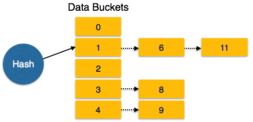
Bucket Overflow

The condition of bucket-overflow is known as collision. This is a fatal state for any static hash function. In this case, overflow chaining can be used.

• Overflow Chaining − When buckets are full, a new bucket is allocated for the same hash result and is linked after the previous one. This mechanism is called Closed Hashing.

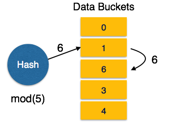
• Linear Probing − When a hash function generates an address at which data is already stored, the next free bucket is allocated to it. This mechanism is called Open Hashing.

Dynamic Hashing

The problem with static hashing is that it does not expand or shrink dynamically as the size of the database grows or shrinks. Dynamic hashing provides a mechanism in which data buckets are added and removed dynamically and on-demand. Dynamic hashing is also known as extended hashing.

Hash function, in dynamic hashing, is made to produce a large number of values and only a few are used initially.

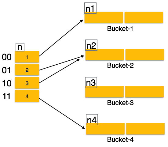
Organization

The prefix of an entire hash value is taken as a hash index. Only a portion of the hash value is used for computing bucket addresses. Every hash index has a depth value to signify how many bits are used for computing a hash function. These bits can address 2n buckets. When all these bits are consumed − that is, when all the buckets are full − then the depth value is increased linearly and twice the buckets are allocated.

Operation

• Querying − Look at the depth value of the hash index and use those bits to compute the bucket address.

• Update − Perform a query as above and update the data.

• Deletion − Perform a query to locate the desired data and delete the same.

• Insertion − Compute the address of the bucket

  • If the bucket is already full.
    • Add more buckets.
    • Add additional bits to the hash value.
    • Re-compute the hash function.
  • Else
    • Add data to the bucket,
  • If all the buckets are full, perform the remedies of static hashing.

Hashing is not favorable when the data is organized in some ordering and the queries require a range of data. When data is discrete and random, hash performs the best.

Hashing algorithms have high complexity than indexing. All hash operations are done in constant time.