Introduction-to Restoration Models

The Imaging model
The image degradation process can be modeled by the following equation:

where, H represents a convolution matrix that models the blurring that many imaging systems introduce. For example, camera defocus, motion blur, imperfections of the lenses all can be modeled by H. The vectors g, f, and w represent the observed, the original and the noise images. More specifically, w is a random vector that models the random errors in the observed data. These errors can be due to the electronics used (thermal and shot noise) the recording medium (film grain) or the imaging process (photon noise).

Problem
Obtaining f from Eq. (1) is not a straight forward task since in most cases of interest the matrix H is ill-posed. Mathematically this means that certain eigenvalues of this matrix are close to zero, which makes the inversion process very unstable. For practical purposes this implies that the inverse or the pseudo-inverse solutions

f₁=H^-1g and f₂=(H^TΗ)^-1Η^Τg (2)

amplify the noise and provide useless results. This fact is demonstrated in what follows.

Solution
Regularization is one way to avoid the problems due to the ill-posed nature of H. According to regularization instead of minimizing || g – Hf ||² in order to find f one minimizes:

|| g – Hf ||² + λ||Qf||² (3)

the additional term ||Qf||² is called regularization term and can be viewed as capturing the properties of the desired solution. In other words, the first term in Eq. (3) stirs the solution f to be “close” to the observed data g while the second term enforces “prior knowledge” to the solution. The prior knowledge that is used is that the image is locally smooth. In most cases Q represents the convolution with a high-pass filter. Thus the term ||Qf||² can be viewed as the high-pass energy of the restored image. The parameter λ is called regularization parameter and controls the closeness to the data vs. the prior knowledge of the solution. Finding f based on Eq. (3) gives

f₃=(H^TH+ λQ^TQ)^-1H^Tg. (4)

Finding the proper value for the parameter λ is an important problem. In the demo that follows one can choose different values of λ and observe the effect to the restored image. A large value of λ results in a smoother image and is necessary if the noise variance is high or H is highly ill-conditioned. On the other hand a large λ blurs out the image details. So one has to decide between smoothness and detail in the solution.

BLIND IMAGE RESTORATION

In many practical cases of interest H is not known. For example when taking the photograph of a moving object when the shutter speed and the speed of the object are unknowns. In this case we are faced with the very difficult problem of “blind” image restoration. In such cases we have to utilize prior knowledge in order to somehow recover simultaneously BOTH f and H. There are many different ways to incorporate prior knowledge about the image f and the degradation H in the problem. One of them is using deterministic constraints in the form of CONVEX SETS, ref [4]. Another approach is using stochastic constraints in the form of prior distributions in a Bayesian framework ref.

For more details on the restoration problem and on the selection regularization the interested reader can go to a number of references that are listed bellow.

REFERENCES
1. M. R. Banham and A. K. Katsaggelos, "Digital Image Restoration,'' IEEE Signal Processing Magazine, vol. 14, no. 2, pp. 24-41, March 1997.

2. D. Kundur and D. Hatzinakos, “Blind Image Deconvolution,” IEEE Signal Processing Magazine, pp. 43-64, May 1997.

3. N. P. Galatsanos and A. K. Katsaggelos, “Methods for Choosing the Regularization Parameter and Estimating the Noise Variance in Image Restoration and their Relation,” IEEE Trans. on Image Processing, Vol. 1, No. 3, pp. 322-336, July 1992.

4. Y. Yang, N. P. Galatsanos, and H. Stark, “Projection Based Blind Deconvolution,” Journal of the Optical Society of America-A, Vol. 11, No. 9, pp. 2401-2409, September 1994.

5. A. Likas, and N. M Galatsanos, “Variational Methods for Bayesian Blind Deconvolution”, Proceedings of the IEEE International Conference on Image Processing (ICIP-03), September Barcelona, Spain 2003.

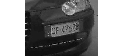
EXAMPLE OF BLIND DECONVOLUTION

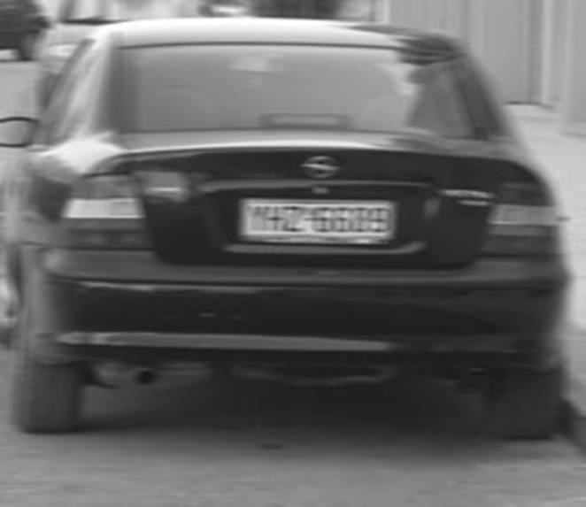
This is an example of the application of blind deconvolution in an image degraded by UNKNOWN blur. Notice the plates of the car in this image are not readable.

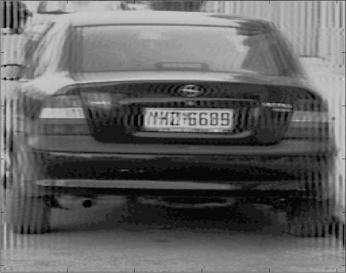
Restored image obtained by 50 iterations of the algorithm in Ref. [5] above.

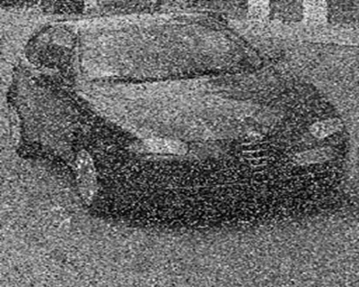
Degraded Image by Film-Grain Noise

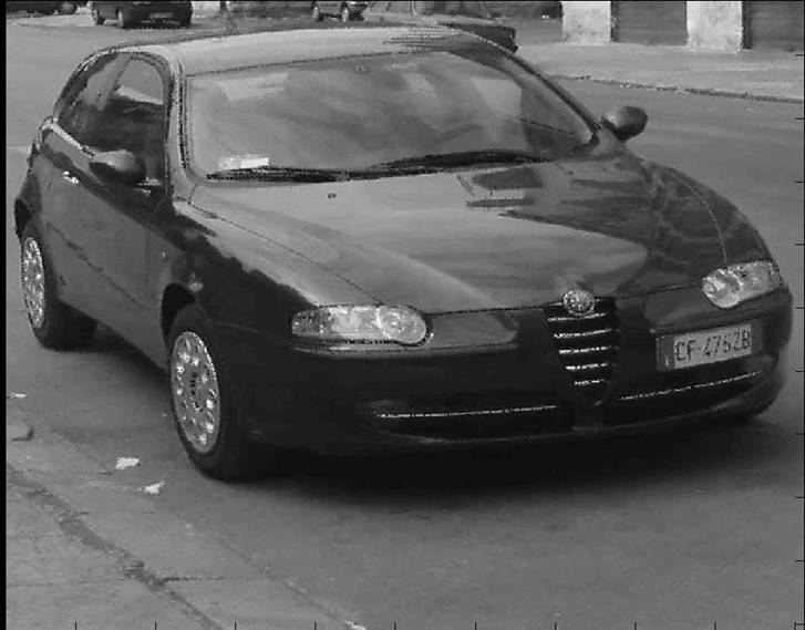
Restored by adaptive window median filter

Area of interest