Theoretical Paper
- Computer Organization
- Data Structure
- Digital Electronics
- Object Oriented Programming
- Discrete Mathematics
- Graph Theory
- Operating Systems
- Software Engineering
- Computer Graphics
- Database Management System
- Operation Research
- Computer Networking
- Image Processing
- Internet Technologies
- Micro Processor
- E-Commerce & ERP
Practical Paper
Industrial Training

Enhancement and segmentation
In the analysis of the objects in images it is essential that we can distinguish between the objects of interest and "the rest." This latter group is also referred to as the background. The techniques that are used to find the objects of interest are usually referred to as segmentation techniques - segmenting the foreground from background. In this section we will two of the most common techniques--thresholding and edge finding-- and we will present techniques for improving the quality of the segmentation result. It is important to understand that:
Thresholding
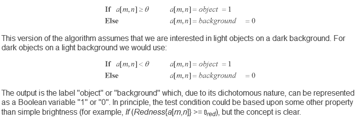
This technique is based upon a simple concept. A parameter called the brightness threshold is chosen and applied to the image a[m,n] as follows:
The central question in thresholding then becomes: ow do we choose the threshold ? While there is no universal procedure for threshold selection that is guaranteed to work on all images, there are a variety of alternatives. * Fixed threshold - One alternative is to use a threshold that is chosen independently of the image data. If it is known that one is dealing with very high-contrast images where the objects are very dark and the background is homogeneous (Section 10.1) and very light, then a constant threshold of 128 on a scale of 0 to 255 might be sufficiently accurate. By accuracy we mean that the number of falsely-classified pixels should be kept to a minimum.
The output is the label "object" or "background" which, due to its dichotomous
nature, can be represented as a Boolean variable "1" or "0". In principle, the
test condition could be based upon some other property than simple brightness
(for example, If (Redness{a[m,n]} >=
red), but the concept is clear.
the central question in thresholding then becomes: ow do we choose the threshold ? while there is no universal procedure for threshold selection that is guaranteed to work on all images, there are a variety of alternatives.
* fixed threshold - one alternative is to use a threshold that is chosen independently of the image data. if it is known that one is dealing with very high-contrast images where the objects are very dark and the background is homogeneous (section 10.1) and very light, then a constant threshold of 128 on a scale of 0 to 255 might be sufficiently accurate. by accuracy we mean that the number of falsely-classified pixels should be kept to a minimum.
* istogram-derived thresholds - in most cases the threshold is
chosen from the brightness histogram of the region or image that we wish to
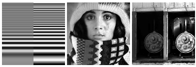
segment. (see sections 3.5.2 and 9.1.) an image and its associated brightness
histogram are shown in figure 51.
a variety of techniques have been devised to automatically choose a threshold starting from the gray-value histogram, {h[b] | b = 0, 1, ... , 2b-1}. some of the most common ones are presented below. many of these algorithms can benefit from a smoothing of the raw histogram data to remove small fluctuations but the smoothing algorithm must not shift the peak positions. this translates into a zero-phase smoothing algorithm given below where typical values for w are 3 or 5:


figure 51: pixels below the threshold (a[m,n] < ) will be labeled as object pixels; those above the threshold will be labeled as background pixels.
* isodata algorithm - this iterative technique for choosing a threshold was developed by ridler and calvard . the histogram is initially segmented into two parts using a starting threshold value such as 0 = 2b-1, half the maximum dynamic range. the sample mean (mf,0) of the gray values associated with the foreground pixels and the sample mean (mb,0) of the gray values associated with the background pixels are computed. a new threshold value 1 is now computed as the average of these two sample means. the process is repeated, based upon the new threshold, until the threshold value does not change any more. in formula:

* background-symmetry algorithm - this technique assumes a distinct and dominant peak for the background that is symmetric about its maximum. the technique can benefit from smoothing as described in eq. . the maximum peak (maxp) is found by searching for the maximum value in the histogram. the algorithm then searches on the non-object pixel side of that maximum to find a p% point as in eq. (39).
in figure 51b, where the object pixels are located to the left of the background peak at brightness 183, this means searching to the right of that peak to locate, as an example, the 95% value. at this brightness value, 5% of the pixels lie to the right (are above) that value. this occurs at brightness 216 in figure 51b. because of the assumed symmetry, we use as a threshold a displacement to the left of the maximum that is equal to the displacement to the right where the p% is found. for figure 51b this means a threshold value given by 183 - (216 - 183) = 150. in formula:

This technique can be adapted easily to the case where we have light objects on a dark, dominant background. Further, it can be used if the object peak dominates and we have reason to assume that the brightness distribution around the object peak is symmetric. An additional variation on this symmetry theme is to use an estimate of the sample standard deviation (s in eq. (37)) based on one side of the dominant peak and then use a threshold based on = maxp +/- 1.96s (at the 5% level) or = maxp +/- 2.57s (at the 1% level). The choice of "+" or "-" depends on which direction from maxp is being defined as the object/background threshold. Should the distributions be approximately Gaussian around maxp, then the values 1.96 and 2.57 will, in fact, correspond to the 5% and 1 % level.
* Triangle algorithm - This technique due to Zack [36] is
illustrated in Figure 52. A line is constructed between the maximum of the
histogram at brightness bmax and the lowest value
bmin = (p=0)% in the image. The distance d
between the line and the histogram h[b] is computed for all
values of b from b = bmin to b =
bmax. The brightness value bo where the
distance between h[bo] and the line is maximal is the
threshold value, that is, = bo. This
technique is particularly effective when the object pixels produce a weak peak
in the histogram.

The triangle algorithm is based on finding the value of b that gives the maximum distance
The three procedures described above give the values θ = 139 for the Isodata algorithm, θ= 150 for the background symmetry algorithm at the 5% level, and = 152 for the triangle algorithm for the image in Figure 51a.
Thresholding does not have to be applied to entire images but can be used on a region by region basis. Chow and Kaneko developed a variation in which the M x N image is divided into non-overlapping regions. In each region a threshold is calculated and the resulting threshold values are put together (interpolated) to form a thresholding surface for the entire image. The regions should be of "reasonable" size so that there are a sufficient number of pixels in each region to make an estimate of the histogram and the threshold. The utility of this procedure--like so many others--depends on the application at hand.
Edge finding
Thresholding produces a segmentation that yields all the pixels that, in
principle, belong to the object or objects of interest in an image. An
alternative to this is to find those pixels that belong to the borders of the
objects. Techniques that are directed to this goal are termed edge
finding techniques. From our discussion in Section 9.6 on
mathematical morphology, specifically eqs. , , and , we see that there is an
intimate relationship between edges and regions.
* Gradient-based procedure - The central challenge to edge finding
techniques is to find procedures that produce closed contours around the
objects of interest. For objects of particularly high SNR, this can be
achieved by calculating the gradient and then using a suitable threshold. This
is illustrated in Figure 53.
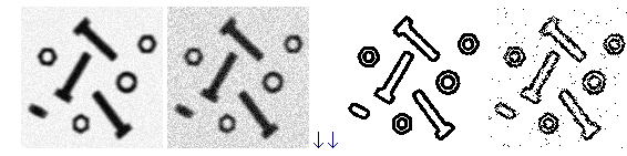
figure 53: edge finding based on the sobel gradient, eq. (110), combined with the isodata thresholding algorithm eq. .
while the technique works well for the 30 db image in figure 53a, it fails to
provide an accurate determination of those pixels associated with the object
edges for the 20 db image in figure 53b. a variety of smoothing techniques as
described in section 9.4 and in eq. can be used to reduce the noise effects
before the gradient operator is applied.
* zero-crossing based procedure - a more modern view to handling the
problem of edges in noisy images is to use the zero crossings generated in the
laplacian of an image (section 9.5.2). the rationale starts from the model of
an ideal edge, a step function, that has been blurred by an otf such as
table 4 t.3 (out-of-focus), t.5 (diffraction-limited), or t.6 (general model)
to produce the result shown in figure 54.
figure 54: edge finding based on the zero crossing as determined by the
second derivative, the laplacian. the curves are not to scale.
the edge location is, according to the model, at that place in the image where
the laplacian changes sign, the zero crossing. as the laplacian operation
involves a second derivative, this means a potential enhancement of noise in
the image at high spatial frequencies; see eq. (114). to prevent enhanced noise
from dominating the search for zero crossings, a smoothing is necessary.
the appropriate smoothing filter, from among the many possibilities described
in section 9.4, should according to canny have the following properties:
* in the spatial domain, (x,y) or [m,n], the filter should be as narrow as possible to provide good localization of the edge. a too wide filter generates uncertainty as to precisely where, within the filter width, the edge is located.
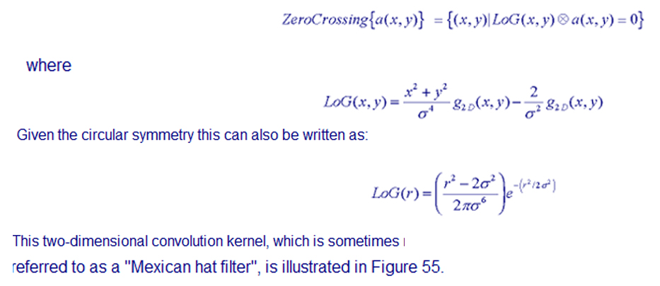
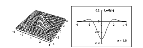
the smoothing filter that simultaneously satisfies both these properties--minimum bandwidth and minimum spatial width--is the gaussian filter described in section 9.4. this means that the image should be smoothed with a gaussian of an appropriate followed by application of the laplacian. in formula:

where g2D(x,y) is defined in eq. (93). The derivative operation is linear and shift-invariant as defined in eqs. (85) and (86). This means that the order of the operators can be exchanged (eq. (4)) or combined into one single filter (eq. (5)). This second approach leads to the Marr-ildreth formulation of the "Laplacian-of-Gaussians" (LoG) filter
neither the derivation of the plus's properties nor an evaluation of its
accuracy are within the scope of this section. suffice it to say that, for
positively curved edges in gray value images, the laplacian-based zero crossing
procedure overestimates the position of the edge and the
sdgd-based procedure underestimates the position. this is true in
both two-dimensional and three-dimensional images with an error on the order of
(/r)2 where r is the radius of
curvature of the edge. the plus operator has an error on the order of
(/r)4 if the image is sampled at, at least,
3x the usual nyquist sampling frequency as in eq. (56) or if we
choose >= 2.7 and sample at the usual nyquist frequency.
All of the methods based on zero crossings in the Laplacian must be able to
distinguish between zero crossings and zero values. While the
former represent edge positions, the latter can be generated by regions that
are no more complex than bilinear surfaces, that is,
a(x,y) = a0 +
a1*x + a2*y +
a3*x*y. To distinguish between these
two situations, we first find the zero crossing positions and label them as "1"
and all other pixels as "0". We then multiply the resulting image by a measure
of the edge strength at each pixel. There are various measures
for the edge strength that are all based on the gradient as described in
Section 9.5.1 and eq. . This last possibility, use of a morphological gradient
as an edge strength measure, was first described by Lee, aralick, and Shapiro
and is particularly effective. After multiplication the image is then
thresholded (as above) to produce the final result. The procedure is thus as
follows :
General strategy for edges based on zero crossings.
The results of these two edge finding techniques based on zero crossings, LoG filtering and PLUS filtering, are shown in Figure 57 for images with a 20 dB SNR.

a) Image SNR = 20 dB ↑ ↓ b) LoG filter c) ↑ ↓ PLUS filter

Edge finding using zero crossing algorithms LoG and PLUS. In both algorithms = 1.5.
Edge finding techniques provide, as the name suggests, an image that contains a collection of edge pixels. Should the edge pixels correspond to objects, as opposed to say simple lines in the image, then a region-filling technique such as eq. may be required to provide the complete objects.
Binary mathematical morphology
The various algorithms that we have described for mathematical morphology in Section 9.6 can be put together to form powerful techniques for the processing of binary images and gray level images. As binary images frequently result from segmentation processes on gray level images, the morphological processing of the binary result permits the improvement of the segmentation result.
* Salt-or-pepper filtering - Segmentation procedures frequently result in isolated "1" pixels in a "0" neighborhood (salt) or isolated "0" pixels in a "1" neighborhood (pepper). The appropriate neighborhood definition must be chosen as in Figure 3. Using the lookup table formulation for Boolean operations in a 3 x 3 neighborhood that was described in association with Figure 43, salt filtering and pepper filtering are straightforward to implement. We weight the different positions in the 3 x 3 neighborhood as follows
For a 3 x 3 window in a[m,n] with values "0" or "1" we then compute:
The result, sum, is a number bounded by 0 <= sum <= 511.
* Salt Filter - The 4-connected and 8-connected versions of this filter are the same and are given by the following procedure:
i) Compute sum ii) If ( (sum == 1) c[m,n] = 0 Else c[m,n] = a[m,n]
* Pepper Filter - The 4-connected and 8-connected versions of this filter are the following procedures:
4-connected 8-connected i) Compute sum i) Compute sum ii) If ( (sum == 170) ii) If ( (sum == 510) c[m,n] = 1 c[m,n] = 1 Else Else c[m,n] = a[m,n] c[m,n] = a[m,n]
* Isolate objects with holes - To find objects with holes we can use the following procedure which is illustrated in Figure 58.
i) Segment image to produce binary mask representation ii) Compute skeleton without end pixels - eq. iii) Use salt filter to remove single skeleton pixels iv) Propagate remaining skeleton pixels into original binary mask - eq.

a) Mask and Seed images b) Objects with holes filled
Figure 59: Filling holes in objects.
The mask image is illustrated in gray in Figure 59a and the seed image is shown in black in that same illustration. When the object pixels are specified with a connectivity of C = 8, then the propagation into the mask (background) image should be performed with a connectivity of C = 4, that is, dilations with the structuring element B = N4. This procedure is also free of "magic numbers."
* Removing border-touching objects - Objects that are connected to the image border are not suitable for analysis. To eliminate them we can use a series of morphological operations that are illustrated in Figure 60.
i) Segment image to produce binary mask image of objects ii) Generate a seed image as the border of the image iv) Propagate the seed into the mask - eq. v) Compute XOR of the propagation result and the mask image as final result

a) Mask and Seed images b) Remaining objects
Figure 60: Removing objects touching borders.
The mask image is illustrated in gray in Figure 60a and the seed image is shown in black in that same illustration. If the structuring element used in the propagation is B = N4, then objects are removed that are 4-connected with the image boundary. If B = N8 is used then objects that 8-connected with the boundary are removed.
* Exo-skeleton - The exo-skeleton of a set of objects is the skeleton of the background that contains the objects. The exo-skeleton produces a partition of the image into regions each of which contains one object. The actual skeletonization (eq. ) is performed without the preservation of end pixels and with the border set to "0." The procedure is described below and the result is illustrated in Figure 61.
i) Segment image to produce binary image ii) Compute complement of binary image iii) Compute skeleton using eq. i+ii with border set to "0"

Exo-skeleton.
* Touching objects - Segmentation procedures frequently have difficulty separating slightly touching, yet distinct, objects. The following procedure provides a mechanism to separate these objects and makes minimal use of "magic numbers." The exo-skeleton produces a partition of the image into regions each of which contains one object. The actual skeletonization is performed without the preservation of end pixels and with the border set to "0." The procedure is illustrated in Figure 62.
i) Segment image to produce binary image ii) Compute a "small number" of erosions with B = N4 iii) Compute exo-skeleton of eroded result iv) Complement exo-skeleton result iii) Compute AND of original binary image and the complemented exo-skeleton

a) Eroded and exo-skeleton images b) Objects separated (detail)
Figure 62: Separation of touching objects.
The eroded binary image is illustrated in gray in Figure 62a and the exo-skeleton image is shown in black in that same illustration. An enlarged section of the final result is shown in Figure 62b and the separation is easily seen. This procedure involves choosing a small, minimum number of erosions but the number is not critical as long as it initiates a coarse separation of the desired objects. The actual separation is performed by the exo-skeleton which, itself, is free of "magic numbers." If the exo-skeleton is 8-connected than the background separating the objects will be 8-connected. The objects, themselves, will be disconnected according to the 4-connected criterion. (See Section 9.6 and Figure 36.)
Gray-value mathematical morphology
As we have seen in Section 10.1.2, gray-value morphological processing techniques can be used for practical problems such as shading correction. In this section several other techniques will be presented.
* Top-hat transform - The isolation of gray-value objects that are convex can be accomplished with the top-hat transform as developed by Meyer . Depending upon whether we are dealing with light objects on a dark background or dark objects on a light background, the transform is defined as:
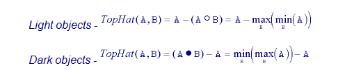
where the structuring element B is chosen to be bigger than the objects in question and, if possible, to have a convex shape. Because of the properties given in eqs. and , Topat(A,B) >= 0. An example of this technique is shown in Figure 63.
The original image including shading is processed by a 15 x 1 structuring element as described in eqs. and to produce the desired result. Note that the transform for dark objects has been defined in such a way as to yield "positive" objects as opposed to "negative" objects. Other definitions are, of course, possible.
* Thresholding - A simple estimate of a locally-varying threshold surface can be derived from morphological processing as follows:

Once again, we suppress the notation for the structuring element B under the max and min operations to keep the notation simple. Its use, however, is understood.


* Local contrast stretching - Using morphological operations we can implement a technique for local contrast stretching. That is, the amount of stretching that will be applied in a neighborhood will be controlled by the original contrast in that neighborhood. The morphological gradient defined in eq. may also be seen as related to a measure of the local contrast in the window defined by the structuring element B:

The max and min operations are taken over the structuring element B. The effect of this procedure is illustrated in Figure 64. It is clear that this local operation is an extended version of the point operation for contrast stretching presented in eq. (77).