Enhancement and segmentation

Image enhancement

The aim of image enhancement is to improve the interpretability or perception of information in images for human viewers, or to provide `better' input for other automated image processing techniques.

Image enhancement techniques can be divided into two broad categories:

1. Spatial domain methods, which operate directly on pixels, and

2. frequency domain methods, which operate on the Fourier transform of an image.

Unfortunately, there is no general theory for determining what is `good' image enhancement when it comes to human perception. If it looks good, it is good! However, when image enhancement techniques are used as pre-processing tools for other image processing techniques, then quantitative measures can determine which techniques are most appropriate.

Spatial domain methodsM

The value of a pixel with coordinates (x,y) in the enhanced image $\hat{F}$ is the result of performing some operation on the pixels in the neighbourhood of (x,y) in the input image, F.
Neighbourhoods can be any shape, but usually they are rectangular.

Grey scale manipulation

The simplest form of operation is when the operator T only acts on a $1 \times 1$ pixel neighbourhood in the input image, that is $\hat{F}(x,y)$ only depends on the value of F at (x,y). This is a grey scale transformation or mapping.

The simplest case is thresholding where the intensity profile is replaced by a step function, active at a chosen threshold value. In this case any pixel with a grey level below the threshold in the input image gets mapped to 0 in the output image. Other pixels are mapped to 255.

Other grey scale transformations are outlined in figure 1 below.

Histogram Equalization

Histogram equalization is a common technique for enhancing the appearance of images. Suppose we have an image which is predominantly dark. Then its histogram would be skewed towards the lower end of the grey scale and all the image detail is compressed into the dark end of the histogram. If we could `stretch out' the grey levels at the dark end to produce a more uniformly distributed histogram then the image would become much clearer.

Histogram equalization involves finding a grey scale transformation function that creates an output image with a uniform histogram (or nearly so).

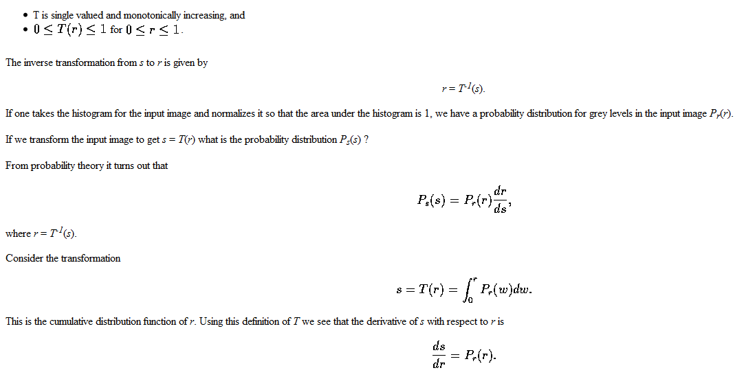
How do we determine this grey scale transformation function? Assume our grey levels are continuous and have been normalized to lie between 0 and 1.

We must find a transformation T that maps grey values r in the input image F to grey values s = T(r) in the transformed image $\hat{F}$.

It is assumed that

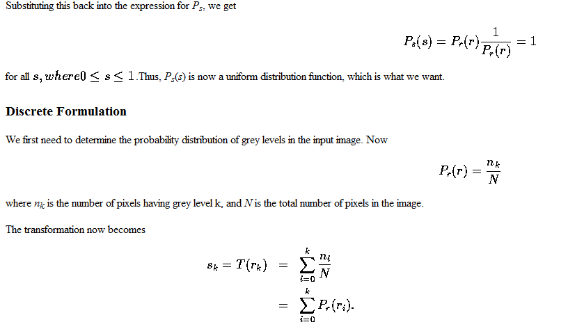
The values of sk will have to be scaled up by 255 and rounded to the nearest integer so that the output values of this transformation will range from 0 to 255. Thus the discretization and rounding of sk to the nearest integer will mean that the transformed image will not have a perfectly uniform histogram.

Image Smoothing

The aim of image smoothing is to diminish the effects of camera noise, spurious pixel values, missing pixel values etc. There are many different techniques for image smoothing; we will consider neighbourhood averaging and edge-preserving smoothing.

Neighbourhood Averaging

Each point in the smoothed image, $\hat{F}(x,y)$ is obtained from the average pixel value in a neighbourhood of (x,y) in the input image.

For example, if we use a $3 \times 3$ neighbourhood around each pixel we would use the mask

1/9 	1/9 	1/9
1/9 	1/9 	1/9
1/9 	1/9 	1/9

Each pixel value is multiplied by $\frac{1}{9}$, summed, and then the result placed in the output image. This mask is successively moved across the image until every pixel has been covered. That is, the image is convolved with this smoothing mask (also known as a spatial filter or kernel).

However, one usually expects the value of a pixel to be more closely related to the values of pixels close to it than to those further away. This is because most points in an image are spatially coherent with their neighbours; indeed it is generally only at edge or feature points where this hypothesis is not valid. Accordingly it is usual to weight the pixels near the centre of the mask more strongly than those at the edge.

Some common weighting functions include the rectangular weighting function above (which just takes the average over the window), a triangular weighting function, or a Gaussian.

In practice one doesn't notice much difference between different weighting functions, although Gaussian smoothing is the most commonly used. Gaussian smoothing has the attribute that the frequency components of the image are modified in a smooth manner.

Smoothing reduces or attenuates the higher frequencies in the image. Mask shapes other than the Gaussian can do odd things to the frequency spectrum, but as far as the appearance of the image is concerned we usually don't notice much

Edge preserving smoothing

Neighbourhood averaging or Gaussian smoothing will tend to blur edges because the high frequencies in the image are attenuated. An alternative approach is to use median filtering. Here we set the grey level to be the median of the pixel values in the neighbourhood of that pixel.

The median m of a set of values is such that half the values in the set are less than m and half are greater. For example, suppose the pixel values in a $3 \times 3$ neighbourhood are (10, 20, 20, 15, 20, 20, 20, 25, 100). If we sort the values we get (10, 15, 20, 20, |20|, 20, 20, 25, 100) and the median here is 20.

The outcome of median filtering is that pixels with outlying values are forced to become more like their neighbours, but at the same time edges are preserved. Of course, median filters are non-linear.

Median filtering is in fact a morphological operation. When we erode an image, pixel values are replaced with the smallest value in the neighbourhood. Dilating an image corresponds to replacing pixel values with the largest value in the neighbourhood. Median filtering replaces pixels with the median value in the neighbourhood. It is the rank of the value of the pixel used in the neighbourhood that determines the type of morphological operation

Image sharpening

The main aim in image sharpening is to highlight fine detail in the image, or to enhance detail that has been blurred (perhaps due to noise or other effects, such as motion). With image sharpening, we want to enhance the high-frequency components; this implies a spatial filter shape that has a high positive component at the centre (see figure 4 below).

A simple spatial filter that achieves image sharpening is given by

-1/9 	-1/9 	-1/9
-1/9 	8/9 	-1/9
-1/9 	-1/9 	-1/9

Since the sum of all the weights is zero, the resulting signal will have a zero DC value (that is, the average signal value, or the coefficient of the zero frequency term in the Fourier expansion). For display purposes, we might want to add an offset to keep the result in the $0 \ldots 255$ range.

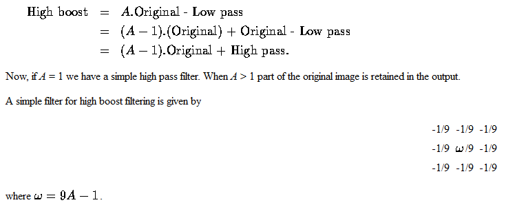
High boost filtering

We can think of high pass filtering in terms of subtracting a low pass image from the original image, that is,

High pass = Original - Low pass.

However, in many cases where a high pass image is required, we also want to retain some of the low frequency components to aid in the interpretation of the image. Thus, if we multiply the original image by an amplification factor A before subtracting the low pass image, we will get a high boost or high frequency emphasis filter. Thus,