Fourier

Brief Description
The Fourier Transform is an important image processing tool which is used to decompose an image into its sine and cosine components. The output of the transformation represents the image in the Fourier or frequency domain, while the input image is the spatial domain equivalent. In the Fourier domain image, each point represents a particular frequency contained in the spatial domain image.

The Fourier Transform is used in a wide range of applications, such as image analysis, image filtering, image reconstruction and image compression

How It Works

As we are only concerned with digital images, we will restrict this discussion to the Discrete Fourier Transform (DFT).

The DFT is the sampled Fourier Transform and therefore does not contain all frequencies forming an image, but only a set of samples which is large enough to fully describe the spatial domain image. The number of frequencies corresponds to the number of pixels in the spatial domain image, i.e. the image in the spatial and Fourier domain are of the same size.

For a square image of size N×N, the two-dimensional DFT is given by:

where f(a,b) is the image in the spatial domain and the exponential term is the basis function corresponding to each point F(k,l) in the Fourier space. The equation can be interpreted as: the value of each point F(k,l) is obtained by multiplying the spatial image with the corresponding base function and summing the result.

The basis functions are sine and cosine waves with increasing frequencies, i.e. F(0,0) represents the DC-component of the image which corresponds to the average brightness and F(N-1,N-1) represents the highest frequency.

In a similar way, the Fourier image can be re-transformed to the spatial domain. The inverse Fourier transform is given by:

Note the Eqn:oneovern2 normalization term in the inverse transformation. This normalization is sometimes applied to the forward transform instead of the inverse transform, but it should not be used for both.$$

To obtain the result for the above equations, a double sum has to be calculated for each image point. However, because the Fourier Transform is separable, it can be written as

Using these two formulas, the spatial domain image is first transformed into an intermediate image using N one-dimensional Fourier Transforms. This intermediate image is then transformed into the final image, again using N one-dimensional Fourier Transforms. Expressing the two-dimensional Fourier Transform in terms of a series of 2N one-dimensional transforms decreases the number of required computations.

Even with these computational savings, the ordinary one-dimensional DFT has Eqn:eqnfour6 complexity. This can be reduced to Eqn:eqnfour5 if we employ the Fast Fourier Transform (FFT) to compute the one-dimensional DFTs. This is a significant improvement, in particular for large images. There are various forms of the FFT and most of them restrict the size of the input image that may be transformed, often to Eqn:eqnfour7 where n is an integer. The mathematical details are well described in the literature.

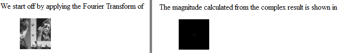
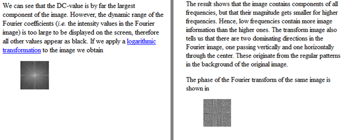
The Fourier Transform produces a complex number valued output image which can be displayed with two images, either with the real and imaginary part or with magnitude and phase. In image processing, often only the magnitude of the Fourier Transform is displayed, as it contains most of the information of the geometric structure of the spatial domain image. However, if we want to re-transform the Fourier image into the correct spatial domain after some processing in the frequency domain, we must make sure to preserve both magnitude and phase of the Fourier image.

The Fourier domain image has a much greater range than the image in the spatial domain. Hence, to be sufficiently accurate, its values are usually calculated and stored in float values.

Guidelines for Use
The Fourier Transform is used if we want to access the geometric characteristics of a spatial domain image. Because the image in the Fourier domain is decomposed into its sinusoidal components, it is easy to examine or process certain frequencies of the image, thus influencing the geometric structure in the spatial domain.

In most implementations the Fourier image is shifted in such a way that the DC-value (i.e. the image mean) F(0,0) is displayed in the center of the image. The further away from the center an image point is, the higher is its corresponding frequency.

shows all frequencies whose magnitude is at least 5% of the main peak. Compared to the original Fourier image, several more points appear. They are all on the same diagonal as the three main components, i.e. they all originate from the periodic stripes. The represented frequencies are all multiples of the basic frequency of the stripes in the spatial domain image. This is because a rectangular signal, like the stripes, with the frequency Eqn:eqnfourb is a composition of sine waves with the frequencies Eqn:eqnfourc, known as the harmonics of Eqn:eqnfourb. All other frequencies disappeared from the Fourier image, i.e. the magnitude of each of them is less than 5% of the DC-value.

A Fourier-Transformed image can be used for frequency filtering. A simple example is illustrated with the above image. If we multiply the (complex) Fourier image obtained above with an image containing a circle (of r = 32 pixels), we can set all frequencies larger than Eqn:eqnfourb to zero as shown in the logarithmic transformed image

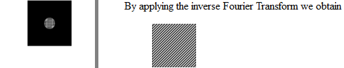
The resulting image is a lowpass filtered version of the original spatial domain image. Since all other frequencies have been suppressed, this result is the sum of the constant DC-value and a sine-wave with the frequency Eqn:eqnfourb. Further examples can be seen in the worksheet on frequency filtering.

A property of the Fourier Transform which is used, for example, for the removal of additive noise, is its distributivity over addition. We can illustrate this by adding the complex Fourier images of the two previous example images. To display the result and emphasize the main peaks, we threshold the magnitude of the complex image, as can be seen in

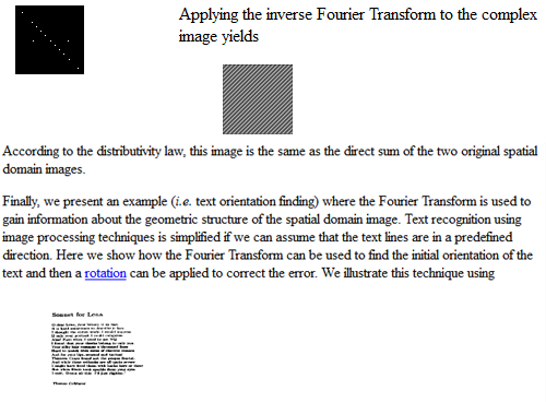
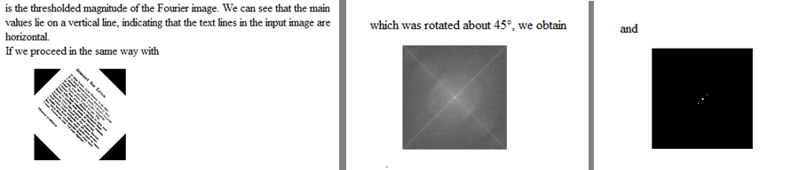
in the Fourier space. We can see that the line of the main peaks in the Fourier domain is rotated according to rotation of the input image. The second line in the logarithmic image (perpendicular to the main direction) originates from the black corners in the rotated image.

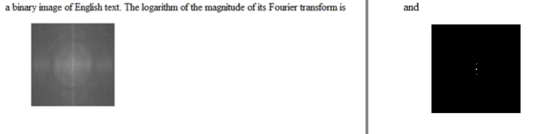
Although we managed to find a threshold which separates the main peaks from the background, we have a reasonable amount of noise in the Fourier image resulting from the irregular pattern of the letters. We could decrease these background values and therefore increase the difference to the main peaks if we were able to form solid blocks out of the text-lines. This could, for example, be done by using a morphological operator.

Common Variants
Another sinusoidal transform (i.e. transform with sinusoidal base functions) related to the DFT is the Discrete Cosine Transform (DCT). For an N×N image, the DCT is given by

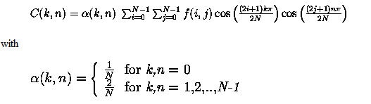
The main advantages of the DCT are that it yields a real valued output image and that it is a fast transform. A major use of the DCT is in image compression --- i.e. trying to reduce the amount of data needed to store an image. After performing a DCT it is possible to throw away the coefficients that encode high frequency components that the human eye is not very sensitive to. Thus the amount of data can be reduced, without seriously affecting the way an image looks to the human eye.

and add them using blend. Take the inverse Fourier Transform of the sum. Explain the result.

Using a paint program, create an image made of periodical patterns of varying frequency and orientation. Examine its Fourier Transform and investigate the effects of removing or changing some of the patterns in the spatial domain image.

Apply the mean operator to

Use the open operator to transform the text lines in the above images into solid blocks. Make sure that the chosen structuring element works for all orientations of text. Compare the Fourier Transforms of the resulting images with the transforms of the unprocessed text images.
Investigate if the Fourier Transform is distributive over multiplication. To do so, multiply

and take the Fourier Transform. Compare the result with the multiplication of the two direct Fourier Transforms.