ML - Support Vector Machine(SVM)

Introduction to SVM

Support vector machines (SVMs) are powerful yet flexible supervised machine learning algorithms which are used both for classification and regression. But generally, they are used in classification problems. In 1960s, SVMs were first introduced but later they got refined in 1990. SVMs have their unique way of implementation as compared to other machine learning algorithms. Lately, they are extremely popular because of their ability to handle multiple continuous and categorical variables.

Working of SVM

An SVM model is basically a representation of different classes in a hyperplane in multidimensional space. The hyperplane will be generated in an iterative manner by SVM so that the error can be minimized. The goal of SVM is to divide the datasets into classes to find a maximum marginal hyperplane (MMH).

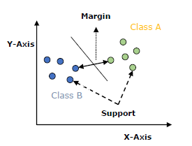
The followings are important concepts in SVM −

• Support Vectors − Datapoints that are closest to the hyperplane is called support vectors. Separating line will be defined with the help of these data points.
• Hyperplane − As we can see in the above diagram, it is a decision plane or space which is divided between a set of objects having different classes.
• Margin − It may be defined as the gap between two lines on the closet data points of different classes. It can be calculated as the perpendicular distance from the line to the support vectors. Large margin is considered as a good margin and small margin is considered as a bad margin.

The main goal of SVM is to divide the datasets into classes to find a maximum marginal hyperplane (MMH) and it can be done in the following two steps −

• First, SVM will generate hyperplanes iteratively that segregates the classes in best way.
• Then, it will choose the hyperplane that separates the classes correctly.

Implementing SVM in Python

• For implementing SVM in Python − We will start with the standard libraries import as follows −

SVM Kernels

In practice, SVM algorithm is implemented with kernel that transforms an input data space into the required form. SVM uses a technique called the kernel trick in which kernel takes a low dimensional input space and transforms it into a higher dimensional space. In simple words, kernel converts non-separable problems into separable problems by adding more dimensions to it. It makes SVM more powerful, flexible and accurate. The following are some of the types of kernels used by SVM.

Linear Kernel

It can be used as a dot product between any two observations. The formula of linear kernel is as below −

                           K(x,xi)=sum(x*xi)

From the above formula, we can see that the product between two vectors say 𝑥 & 𝑥𝑖 is the sum of the multiplication of each pair of input values.

Polynomial Kernel

It is more generalized form of linear kernel and distinguish curved or nonlinear input space. Following is the formula for polynomial kernel −

                          k(X,Xi)=1+sum(X∗Xi)^d

Here d is the degree of polynomial, which we need to specify manually in the learning algorithm.

Radial Basis Function (RBF) Kernel

		     K(x,xi)=exp(−gamma∗sum(x−xi^2))

Here, gamma ranges from 0 to 1. We need to manually specify it in the learning algorithm. A good default value of gamma is 0.1.

As we implemented SVM for linearly separable data, we can implement it in Python for the data that is not linearly separable. It can be done by using kernels.