Curves and their presentations

In the mathematical subfield of numerical analysis a Bézier curve is a parametric curve important in computer graphics. A numerically stable method to evaluate Bézier curves is de Casteljau's algorithm. Generalizations of Bézier curves to higher dimensions are called Bézier surfaces, of which the Bézier triangle is a special case.
Bézier curves were widely publicized in 1962 by the French engineer Pierre Bézier who used them to design automobile bodies. The curves were developed in 1959 by Paul de Casteljau using de Casteljau's algorithm.

TrueType fonts use Bézier splines composed of the quadratic Bézier curves.

Cubic Bézier curvesEdit
File:Bezier.png
Four points P0, P1, P2 and P3 in the plane or in three-dimensional space define a cubic Bézier curve. The curve starts at P0 going toward P1 and arrives at P3 coming from the direction of P2. In general, it will not pass through P1 or P2; these points are only there to provide directional information. The distance between P0 and P1 determines "how long" the curve moves into direction P2 before turning towards P3.

The parametric form of the curve is:
\mathbf{B}(t)=\mathbf{P}_0(1-t)^3+3\mathbf{P}_1t(1-t)^2+3\mathbf{P}_2t^2(1-t)+\mathbf{P}_3t^3 \mbox{ , } t \in [0,1]. Modern imaging systems like PostScript, Metafont and GIMP use Bézier splines composed of cubic Bézier curves for drawing curved shapes.

Generalization

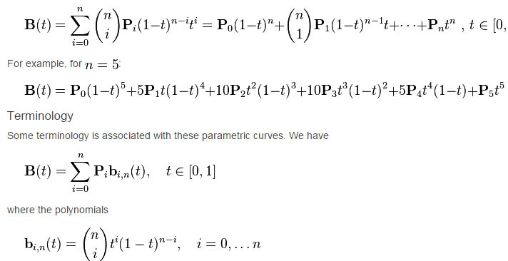
The points Pi are called control points for the Bézier curve. The polygon formed by connecting the Bézier points with lines, starting with P0 and finishing with Pn, that is, the convex hull of the Pi , is called the Bézier polygon, and the Bézier polygon contains the Bézier curve.

Notes Edit
The curve begins at P0 and ends at Pn; this is the so-called endpoint interpolation property.
The curve is a straight line if and only if all the control points lie on the curve, similarly, the Bézier curve is a straight line if and only if the control points are collinear
The start (end) of the curve is tangent to the first (last) section of the Bézier polygon.
A curve can be split at any point into 2 subcurves, or into arbitrarily many subcurves, each of which is also a Bézier curve.
A circle cannot be exactly formed by a Bézier curve, not even a circular arc. However, often a Bézier curve is an adequate approximation to a small enough circular arc.
The curve at a fixed offset from a given Bézier curve ("parallel" to that curve, like the offset between rails in a railroad track) cannot be exactly formed by a Bézier curve (except in some trivial cases). However, there are heuristic methods that usually give an adequate approximation for practical purposes.

Application in computer graphicsEdit

Bézier curves are widely used in computer graphics to model smooth curves. As the curve is completely contained in the convex hull of its control points, the points can be graphically displayed and used to manipulate the curve intuitively. Affine transformations such as translation, scaling and rotation can be applied on the curve by applying the respective transform on the control points of the curve.
The most important Bézier curves are quadratic and cubic curves. Higher degree curves are more expensive to evaluate. When more complex shapes are needed low order Bézier curves are patched together (obeying certain smoothness conditions) in the form of Bézier splines.

Code example Edit

The following code is a simple practical example showing how to plot a cubic Bezier curve in the C programming language. Note, this simply computes the coefficients of the polynomial and runs through a series of t values from 0 to 1 -- in practice this is how it is usually done, even though algorithms such as de Casteljau's are often cited in graphics discussions, etc. This is because in practice a linear algorithm like this is faster and less resource-intensive than a recursive one like de Casteljau's. The following code has been factored to make its operation clear - an optimization in practice would be to compute the coefficients once and then re-use the result for the actual loop that computes the curve points - here they are recomputed every time, which is less efficient but helps to clarify the code.

The resulting curve can be plotted by drawing lines between successive points in the curve array - the more points, the smoother the curve.

On some architectures, the code below can also be optimized by dynamic programming. E.g. since dt is constant, cx * t changes a constant amount with every iteration. By repeatedly applying this optimization, the loop can be rewritten without any multiplications (though such a procedure is not numerically stable).

/*
Code to generate a cubic Bezier curve
*/

typedef struct
{
    float x;
    float y;
}
Point2D;

/*
cp is a 4 element array where:
cp[0] is the starting point, or A in the above diagram
cp[1] is the first control point, or B
cp[2] is the second control point, or C
cp[3] is the end point, or D
t is the parameter value, 0 <= t <= 1
*/

Point2D PointOnCubicBezier( Point2D* cp, float t )
{
    float   ax, bx, cx;
    float   ay, by, cy;
    float   tSquared, tCubed;
    Point2D result;

    /* calculate the polynomial coefficients */

    cx = 3.0 * (cp[1].x - cp[0].x);
    bx = 3.0 * (cp[2].x - cp[1].x) - cx;
    ax = cp[3].x - cp[0].x - cx - bx;
	
    cy = 3.0 * (cp[1].y - cp[0].y);
    by = 3.0 * (cp[2].y - cp[1].y) - cy;
    ay = cp[3].y - cp[0].y - cy - by;
	
    /* calculate the curve point at parameter value t */
	
    tSquared = t * t;
    tCubed = tSquared * t;
	
    result.x = (ax * tCubed) + (bx * tSquared) + (cx * t) + cp[0].x;
    result.y = (ay * tCubed) + (by * tSquared) + (cy * t) + cp[0].y;
	
    return result;
}

/*
 ComputeBezier fills an array of Point2D structs with the curve   
 points generated from the control points cp. Caller must 
 allocate sufficient memory for the result, which is 
 
*/

void ComputeBezier( Point2D* cp, int numberOfPoints, Point2D* curve ) {
    float   dt;
    int	  i;

    dt = 1.0 / ( numberOfPoints - 1 );

    for( i = 0; i < numberOfPoints; i++)
    curve[i] = PointOnCubicBezier( cp, i*dt );
}

Another application for Bézier curves is to describe paths for the motion of objects in animations, etc. Here, the x, y positions of the curve are not used to plot the curve but to position a graphic. When used in this fashion, the distance between successive points can become important, and in general these are not spaced equally - points will cluster more tightly where the control points are close to each other, and spread more widely for more distantly positioned control points. If linear motion speed is required, further processing is needed to spread the resulting points evenly along the desired path.

Rational Bézier curves

Some curves that seem simple, like the circle, cannot be described by a Bézier curve or a piecewise Bézier curve (though in practice the difference is small and may be tolerable). To describe some of these other curves, we need additional degrees of freedom.

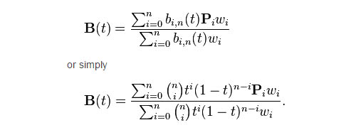
The rational Bézier curve adds weights that can be adjusted. The numerator is a weighted Bernstein form Bézier curve and the denominator is a weighted sum of Bernstein polynomials.

Given n + 1 control points Pi, the rational Bézier curve can be described by: