Space Time

Landau's symbols O and Θ
Making predictions on the running time and space consumption of a program
Amortized analysis

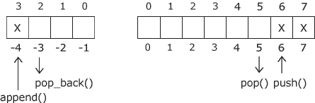
In Section 2.2.1 we implemented a simple sorting algorithm, sorting by minimum search. We used it there to sort characters; we also could sort numbers or strings with it because it is only based on comparisons and swapping. All we have to do to sort strings with the same algorithm is to replace the type name array in the source code by array... and we can sort a complete phone book: the phone book of Saarbrücken, of Munich, of Germany. Can we really?

Time complexity

How long does this sorting program run? It possibly takes a very long time on large inputs (that is many strings) until the program has completed its work and gives a sign of life again. Sometimes it makes sense to be able to estimate the running time before starting a program. Nobody wants to wait for a sorted phone book for years! Obviously, the running time depends on the number n of the strings to be sorted. Can we find a formula for the running time which depends on n?

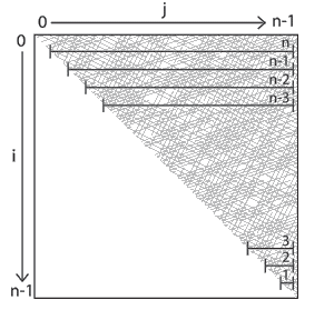
Having a close look at the program we notice that it consists of two nested for-loops. In both loops the variables run from 0 to n, but the inner variable starts right from where the outer one just stands. An if with a comparison and some assignments not necessarily executed reside inside the two loops. A good measure for the running time is the number of executed comparisons.[11] In the first iteration n comparisons take place, in the second n-1, then n-2, then n-3 etc. So 1+2+...+n comparisons are performed altogether. According to the well known Gaussian sum formula these are exactly 1/2·(n-1)·n comparisons. Figure 2.8 illustrates this. The screened area corresponds to the number of comparisons executed. It apparently corresponds approx. to half of the area of a square with a side length of n. So it amounts to approx. 1/2·n2.

Running time analysis of sorting by minimum search

How does this expression have to be judged? Is this good or bad? If we double the number of strings to be sorted, the computing time quadruples! If we increase it ten-fold, it takes even 100 = 102 times longer until the program will have terminated! All this is caused by the expression n2. One says: Sorting by minimum search has quadratic complexity. This gives us a forefeeling that this method is unsuitable for large amounts of data because it simply takes far too much time.

So it would be a fallacy here to say: “For a lot of money, we'll simply buy a machine which is twice as fast, then we can sort twice as many strings (in the same time).” Theoretical running time considerations offer protection against such fallacies.

The number of (machine) instructions which a program executes during its running time is called its time complexity in computer science. This number depends primarily on the size of the program's input, that is approximately on the number of the strings to be sorted (and their length) and the algorithm used. So approximately, the time complexity of the program “sort an array of n strings by minimum search” is described by the expression c·n2.

c is a constant which depends on the programming language used, on the quality of the compiler or interpreter, on the CPU, on the size of the main memory and the access time to it, on the knowledge of the programmer, and last but not least on the algorithm itself, which may require simple but also time consuming machine instructions. (For the sake of simplicity we have drawn the factor 1/2 into c here.) So while one can make c smaller by improvement of external circumstances (and thereby often investing a lot of money), the term n2, however, always remains unchanged.

The O-notation

In other words: c is not really important for the description of the running time! To take this circumstance into account, running time complexities are always specified in the so-called O-notation in computer science. One says: The sorting method has running time O(n2). The expression O is also called Landau's symbol.

Mathematically speaking, O(n2) stands for a set of functions, exactly for all those functions which, “in the long run”, do not grow faster than the function n2, that is for those functions for which the function n2 is an upper bound (apart from a constant factor.) To be precise, the following holds true: A function f is an element of the set O(n2) if there are a factor c and an integer number n0 such that for all n equal to or greater than this n0 the following holds:

f(n) ≤ c·n².

The function n² is then called an asymptotically upper bound for f. Generally, the notation f(n)=O(g(n)) says that the function f is asymptotically bounded from above by the function

A function f from O(n²) may grow considerably more slowly than n² so that, mathematically speaking, the quotient f / n² converges to 0 with growing n. An example of this is the function f(n)=n. However, this does not hold for the function f which describes the running time of our sorting method. This method always requires n² comparisons (apart from a constant factor of 1/2). n² is therefore also an asymptotically lower bound for f. This f behaves in the long run exactly like n². Expressed mathematically: There are factors c₁ and c₂ and an integer number n₀ such that for all n equal to or larger than n₀ the following holds:

c₁·n² ≤ f(n) ≤ c₂·n².
So f is bounded by n² from above and from below. There also is a notation of its own for the set of these functions: Θ(n²).

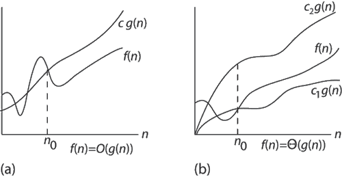contrasts a function f which is bounded from above by O(g(n)) to a function whose asymptotic behavior is described by Θ(g(n)): The latter one lies in a tube around g(n), which results from the two factors c₁ and c₂.

These notations appear again and again in the LEDA manual at the description of non-trivial operations. Thereby we can estimate the order of magnitude of the method used; in general, however, we cannot make an exact running time prediction. (Because in general we do not know c, which depends on too many factors, even if it can often be determined experimentally;

Frequently the statement is found in the manual that an operation takes “constant time”. By this it is meant that this operation is executed with a constant number of machine instructions, independently from the size of the input. The function describing the running time behavior is therefore in O(1). The expressions “linear time” and “logarithmic time” describe corresponding running time behaviors: By means of the O-notation this is often expressed as “takes time O(n) and O(log(n))”, respectively.

Furthermore, the phrase “expected time” O(g(n)) often appears in the manual. By this it is meant that the running time of an operation can vary from execution to execution, that the expectation value of the running time is, however, asymptotically bounded from above by the function g(n).

Back to our sorting algorithm: A runtime of Θ(n2) indicates that an adequately big input will always bring the system to its knees concerning its running time. So instead of investing a lot of money and effort in a reduction of the factor c, we should rather start to search for a better algorithm. Thanks to LEDA, we do not have to spend a long time searching for it: All known efficient sorting methods are built into LEDA.

To give an example, we read on the manual page of array in the section “Implementation” that the method sort() of arrays implements the known Quicksort algorithm whose (expected) complexity is O(n·log(n)) which (seen asymptotically) is fundamentally better than Θ(n2). This means that Quicksort defeats sorting by minimum search in the long run: If n is large enough, the expression c1·n·log(n) certainly becomes smaller than the expression c2·n2, independently from how large the two system-dependent constants c1 and c2 of the two methods actually are; the quotient of the two expressions converges to 0. (For small n, however, c1·n·log(n) may definitely be larger than c2·n2; indeed, Quicksort does not pay on very small arrays compared to sorting by minimum search.)

Now back to the initial question: Can we sort phone books with our sorting algorithm in acceptable time? This depends, in accordance to what we said above, solely on the number of entries (that is the number of inhabitants of the town) and on the system-dependent constant c. Applied to today's machines: the phone book of Saarbrücken in any case, the one of Munich maybe in some hours, but surely not the one of Germany. With the method sort() of the class array, however, the last problem is not a problem either.

Space complexity
The better the time complexity of an algorithm is, the faster the algorithm will carry out his work in practice. Apart from time complexity, its space complexity is also important: This is essentially the number of memory cells which an algorithm needs. A good algorithm keeps this number as small as possible, too.

There is often a time-space-tradeoff involved in a problem, that is, it cannot be solved with few computing time and low memory consumption. One then has to make a compromise and to exchange computing time for memory consumption or vice versa, depending on which algorithm one chooses and how one parameterizes it.

Amortized analysis
Sometimes we find the statement in the manual that an operation takes amortized time O(f(n)). This means that the total time for n such operations is bounded asymptotically from above by a function g(n) and that f(n)=O(g(n)/n). So the amortized time is (a bound for) the average time of an operation in the worst case.

The special case of an amortized time of O(1) signifies that a sequence of n such operations takes only time O(n). One then refers to this as constant amortized time.

Such statements are often the result of an amortized analysis: Not each of the n operations takes equally much time; some of the operations are running time intensive and do a lot of “pre-work” (or also “post-work”), what, however, pays off by the fact that, as a result of the pre-work done, the remaining operations can be carried out so fast that a total time of O(g(n)) is not exceeded. So the investment in the pre-work or after-work amortizes itself.

Exercise 8.	Create an array of 10,000 integer numbers. Sort it with the algorithm from Measure the running time and determine the factor c experimentally therewith. Based on this, make predictions how long the sorting of an array with 100,000 (Saarbrücken) elements, 1,000,000 elements (Munich), and 10,000,000 elements (Germany) will take. Test your prediction for an array consisting of 1,000,000 elements. Then replace the algorithm by LEDA's sort() method and measure the running times once more. Hint: The function used_time(), which is described in , offers its services for measuring running times.
Exercise 9.	Another sorting method which also takes only time O(n·log((n)) is Mergesort. It works recursively: One divides the array to be sorted into two halves, sorts each of the two halves recursively, and then merges the sorted halves to a sorted array. What does it mean to “merge”? Merging is performed by pairwise comparing the elements of the two subarrays already sorted. Two index variables are used here, which run from left to right over the subarrays to be merged. The respectively smaller (or larger in a descending sorting) element is written into a temporary array. The index variable pointing to the smaller of the two values is advanced by one position to the right. Work out the details. Why does this method always take only time O(n·log(n))? Implement this method and let it compete with LEDA's sort() and sorting by minimum search.
Exercise 10.	To append arbitrarily many elements at one end of an array, the following doubling strategy can be used: Every time the array is full, its size is doubled by means of resize(). Work out why appending an element takes amortized time O(1) with this doubling strategy and therefore takes not considerably longer than appending an element at one end of a linear list. (There, each and every insert and delete takes guaranteed time O(1), at whatever position it is performed, Work out why this does not hold if the elements are inserted at the front or in the middle of the array (in contrast to inserting into a linear list). Therefore, appending n elements to an initially empty array takes time O(n) with this doubling strategy. Compare this to the time it takes if the array size grows by 1 with every single append and all elements have to be copied to a new location.
Exercise 11.	In < we will get to know queues; a queue is a data structure in which elements can be appended at one end and extracted at the other end only. In contrast, elements can be inserted and extracted at both ends of a deque (“double ended queue”, pronounced as “deck”), see A deque is a queue in which elements can be inserted and extracted at both ends. This deque is implemented by two arrays A and B. It contains 9 elements. The elements at the two ends are the elements A[2] and B[5]. The figure points out at which position the next pop(), push() append(), or pop_back(), respectively, will modify the deque. LEDA does not have a class deque, because, among other reasons, such a structure is only rarely needed and can be easily simulated by a linear list or a clever arrangement of two arrays. Write a class deque which implements a deque. Inserting and deleting an element shall be possible in amortized time O(1) at both ends. Every element shall in addition be accessible in constant time via an index. (A linear list therefore is out of question for the implementation; gives a hint for the solution of the problem.)