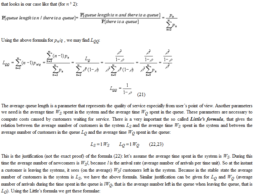
The M/M/1 Queuing System

The M/M/1 system is made of a Poisson arrival, one exponential (Poisson) server, FIFO (or not specified) queue of unlimited capacity and unlimited customer population. Note that these assumptions are very strong, not satisfied for practical systems (the worst assumption is the exponential distribution of service duration - hardly satisfied by real servers). Nevertheless the M/M/1 model shows clearly the basic ideas and methods of Queuing Theory. Next two chapters summarize the basic properties of the Poisson process and give derivation of the M/M/1 theoretical model.

poisson process

1) p[one arrival in the time interval (t, t+h), for h ® 0] = lh, where l is a constant.

2) p[more than one arrivals in the interval (t, t+h), for h ® 0] ® 0.

3) the above probabilities do not depend on t ("no memory" property = time independence = stationarity).

let p_n(t) = p[n arrivals in the time interval (0, t)]. using the above assumptions 1) and 2), it is possible to express the probability p_n(t+h), h ® 0:

p_n(t+h) = p_n(t) [1 - lh] + p_n-1(t)l h
( n arrivals by t, no more arrival or n-1 arrivals by t, one more arrival)

p₀(t+h) = p₀(t)[1 - lh]
( no arrival by t, no more arrival)    (1)

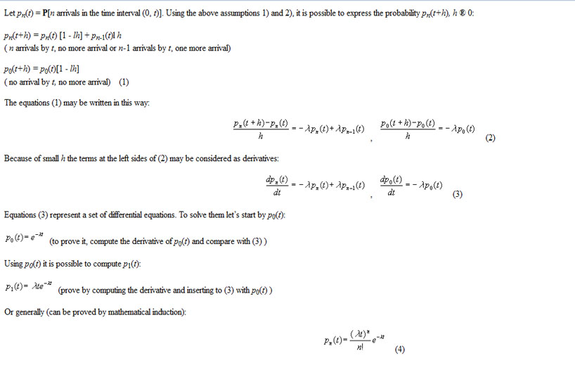
Because of the assumption 3) the formula (4) holds for any interval (s, s+t), in other words the probability of n arrivals during some time interval depends only on the length of this time interval (not on the starting time of the interval).

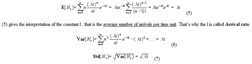
Number of arrivals Nt during some time interval t is a discrete random variable associated with the Poisson process. Having the probabilities of the random values - (4), it is possible to find the usual parameters of the random variable Nt. Let E[x] be the mean (average) value, Var[x] the variance, and Std[x] the standard deviation of the random variable x:

Another random variable associated with the Poisson process is the random interval between two adjacent arrivals. Let x be the random interval. To find its distribution, let’s express the Distribution function F(x):

F(x) = P[interval < x] = P[at least one arrival during the interval x] = 1 - p0(x) = 1 - e-l x

Because the interval is a continuous random variable, it is possible to compute the Probability density as a derivative of the Distribution function:

f(x) = dF(x)/dx = l e-l x

These two functions define the probability distribution:

f(x) = 1 - e^{-l x}  ,  f(x) = l e^{-l x}    (8)

The distribution (8) is called Exponential or Negative Exponential Distribution. Its parameters are:

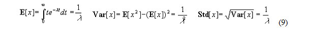
(9) gives another interpretation of the constant l . Its inverted value is the average interval between arrivals. Like the number of arrivals, the distribution of intervals between arrivals does not depend on time. Note the big value of the standard deviation (equal to the average value). It means, that the exponential distribution is "very random". In fact all intervals from 0 to ¥ are theoretically possible. So it may happen, that there will be clusters of very close arrivals separated by very long intervals. Of course not all practical distributions can be treated as exponential ones. There is this general rule:

If a large number of independent event streams are merged together, and if events in each stream occur at a very low rate, then the resulting stream is approximately a Poisson process with exponential intervals.

This rule is more or less satisfied for arrivals in systems with large populations (each potential customer represents one low rate stream).

When applied to a service, the rate is called Service rate (m ). The parameter m is the average number of completed services per time unit (provided there are always customers waiting in the queue), its inverted value 1/m is the average duration of the exponential service. The variance and the standard deviation can be computed by replacing l by m in the formulae (9). Unlike arrival, exponential service is an abstraction that is hardly satisfied by real systems, because mostly it is very unlikely to have very short and/or very long services. Real service duration will be typically "less random" than the theoretical exponential distribution.

Another very important parameter of queuing systems is the ratio r of the arrival and the service rates called Traffic rate (sometimes called Traffic intensity or Utilisation factor):

the m/m/1 system is made of a poisson arrival (arrival rate l ), one exponential server (service rate m ), unlimited fifo (or not specified queue), and unlimited customer population. because both arrival and service are poisson processes, it is possible to find probabilities of various states of the system, that are necessary to compute the required quantitative parameters. system state is the number of customers in the system. it may be any nonnegative integer number. let p_n(t) = p[n customers in the system at time t]. like with the poisson process, by using the assumptions 1) and 2), it is possible to express the probability p_n(t+h), h ® 0 in this way:

p_n(t+h) = p_n(t)[1 - lh][1 - mh] +        (n customers at t, no came, no left)

p_n(t)[lh][mh] +        (n customers at t, one came, one left)

p_n-1(t)[lh][1 - mh] +        (n-1 customers at t, one came, no left)

p_n+1(t)[1 - lh][mh]         (n+1 customers at t, no came, one left )

p₀(t+h) = p₀(t)[1 - lh] +        (no customer at t, no came)

p₁(t)[1 - lh][mh]        (one customer at t, no came, one left)    (11)

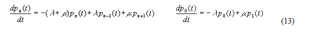
the above equations may be written in the following way, where the terms with h² are omitted because they are relatively very small ( h ® 0):

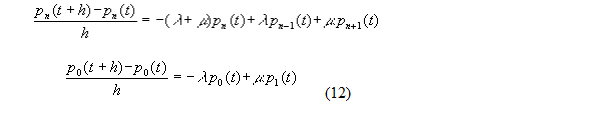
Because of small h the terms at the left sides of (12) may be considered as derivatives: