Dynamic Programming Characteristics

Dynamic programming is basically a mathematical technique developed by Richard Bellman and his associates at the Rand Corporation. This technique is a powerful tool for making a sequence of interrelated decisions. There is no standard mathematical formulation of the dynamic programming problem, which is in

Operations Research (MTH601)

contrast to linear programming. It is a general type of approach to problem solving and each problem has to be analyzed depending on the conditions pertaining to the problem and the particular equations used must be developed to suit the problem. In this way one should take care to formulate a dynamic programming problem, using the method of recursion.

Dynamic programming provides a solution with much less effort than exhaustive enumeration. In dynamic programming we start with a small portion of the problem and find the optimal solution for this smaller problem. We then gradually enlarge the problem finding the current optimal solution from the previous one, until we solve the original problem in its entirety. In this connection we refer to Bellman's principle of optimality, which states:

"An optimal policy has the property that, whatever the initial state and initial decision are, the remaining decisions must constitute an optimal policy with respect to the state resulting from the first decision". Dynamic programming technique can be applied to problems of inventory control, production planning, chemical reactor design, heat exchanger designs, business situation to take an optimal decision for investments etc.

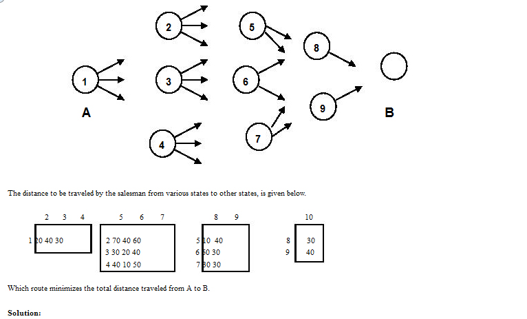
A number of illustrative examples are presented for developing dynamic programming procedure. We consider the following problem called "Stage coach problem" to illustrate the concepts of Example

dynamic programming. A salesman has to travel between points A to B indicated by the network shown in

Operations Research (MTH601)

First point we note in this problem is that the decision, which is best for each successive stage, need not yield the over-all optimal decision. If we follow the policy of minimum distance at each state, we land in a path A→2→6→9→B, with a total distance travelled as 130 km. However it should be evident that sacrificing a little on one is less distant that A→2→6 = (2 + 4).

We can solve the problem by trial and error. The number of possible routes is 18 in this example and having to calculate the total distance for all routes is a tiresome task. Instead of exhaustive enumeration of all the routes, it is better to start with a small problem and find the optimal solution for this smaller problem. Thus we extend this for the entire problem. This is what we try to do in dynamic programming. The problem is divided into a number of stages and proceeds backwards from final destination. In this example if we were in 8 or 9 and the final destination is B we have to travel only one stage to complete the journey. This we call as one stage problem indicating that there is one more stage to go to complete the journey. If we were in 5 or 6 or 7 we have to travel 2 stages to reach the final destination. Like this we have 4 stages from A to B.

Let xn(n = 1, 2, 3, 4) be the immediate destination when there are n more stages to travel. Thus, the route selected would be 1→x4→x3→x2→x1, where x1 = 10. Let fn(x, xn) be the total cost of the best over-all policy for the last n stages, given that the salesman is in the state s and selects xn as the immediate destination called the state. Given s and n, let xn* denote the value of xn which minimizes fn(s1, xn), and let fn*(s) be the corresponding minimum value of fn(x, xn). Thus, fn*(s) = fn(s, xn*). The objective is to find f4*(1) and the corresponding policy. In dynamic programming we successively find f1*(s), f2*(s), f3*(s) and f4*(1). The problem is divided into four stages. In one stage problem, we have one more stage to go, we can write the solution to one-stage problem as follows

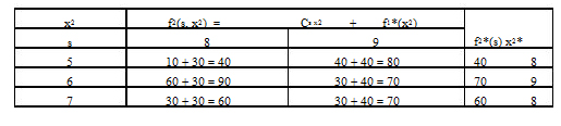
When the salesman has two more stages to go, the solution requires a little analysis. When two stages are ahead to reach final destination he may occupy one of the states 5 or 6 or 7. If he is in state 5, he must go to either state 8 or 9 at a cost of 10 or 40 respectively. If he selects state 8, the minimum additional distanced to travel after reaching there, is given in the above table as 30 so that the total distance for this decision would be 10 + 30 = 40. If he selects state 9, the total distance is 40 + 40 = 80. Comparing the two cases, it is better if he would choose 8, x2* = 8, since it gives the minimum total distance, f2*(5) = 40. In the same way for s = 6 and s = 7, we get the following results for the two stage problem shown below

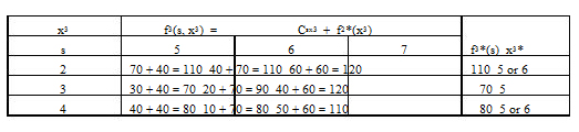
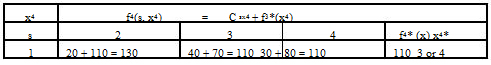
The solution for the three-stage problem is obtained in a similar fashion. In the three-stage problem, we have f3(s, x3) = Csx3 + f2*(x3). To illustrate, if the salesman is in state 2, and selects to go to state 5 next, the minimum total distance, f3(2, 5) would be the cost of the first stage C25 = 70 plus the minimum distance from state 5 onward f2*(5) = 4 so that f3*(2, 5) = 70 + 40 = 110, similarly f5*(2, 6) = 40 + 70 = 110 and f3*(2, 7) = 60

Operations Research (MTH601) 262 + 60 = 120, so that the minimum total distance from state 2 onward is f3*(2) = 110 and the immediate destination should be x3* = 5 or 6. The results are tabulated below

Continuing in this way, we move to the four-stage problem. The optimum distance travelled given the immediate destination, is again the sum of the distances of the first stage plus the minimum distance thereafter. The results are tabulated in table

We can summarize the optimal solution. From the four stage problem, we infer that the salesman should go initially to either state 3 or state 4. If he chooses x4* = 3, the three-stage problem result for s = 3 is x4* = 5. From this we go to the two stage problem which gives x*2 = 8 for s = 5 and the single stage problem yields x1* = 10 for s = 8. Hence the optimal route is 1→3→5→8→10. If the salesman selects x4*=4, this leads to the other two optimal routes, 1→4→5→8→10 and 1→4→6→9→10. They all yield a total of f4*(1) = 110

FEATURES CHARECTERIZING DYNAMIC PROGRAMMING PROBLEMS

The physical interpretation to the abstract structure of dynamic programming problems can be provided by the example of stagecoach problem discussed in the previous section. Any problem in dynamic programming can be formulated with its basic structure similar to that of the stagecoach problem. The basic features, which characterize dynamic programming problems, are given in the following.
1. The problem can be divided up into stages, with a policy decision required at each stage.
2. Each stage has a number of states associated with it.
3. The effect of the policy decision at each stage is to change the current state into a state associated with the next stage.
4. Given the current state, an optimal policy for the remaining stage, is independent of the policy adopted in previous stages.
5. The procedure of solving the problem begins by finding the optimal policy for each state of the last stage.
6. A recursive formula can be framed to identify the optimal policy for each state with (n - 1) stages remaining.
7. Using the recursive relationship the procedure is to move backward stage by stage, until it finds the optimal policy when starting at the initial stage.

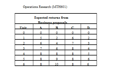
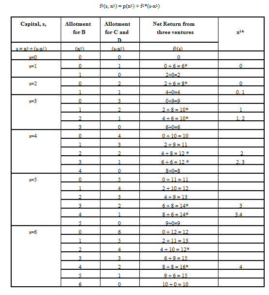
The problem has 4 stages, each business proposal representing a stage and we have six states Solution:
with each stage.
One stage problem
Here we consider only one business proposal namely D (working backward) we can allot any unit of capital and the expected returns are as shown in table. For business D alone

Here we consider two business proposals D and C. The capital is to be allocated to D and C in many possible ways. If a certain unit of capital is allotted to C (second new business) then the remaining capital only can be allocated to D and we have several combinations. The convenient way to understand about the returns is to analyse all possible combinations. Let x1, be the amount allotted to D and x2 to C

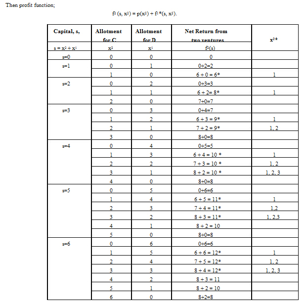
Now we turn to a three-stage problem. Here we consider three business ventures. The capital can be allotted to business venture B (= x3) and the remaining amount to C and D combined